When working with algorithms and data structures, efficiency often comes down to how quickly you can retrieve the information you need. One of the most powerful tools to achieve this is the Lookup Table. Let’s break down what it is, why we need it, when to use it, and the performance considerations behind it.
What is a Lookup Table?
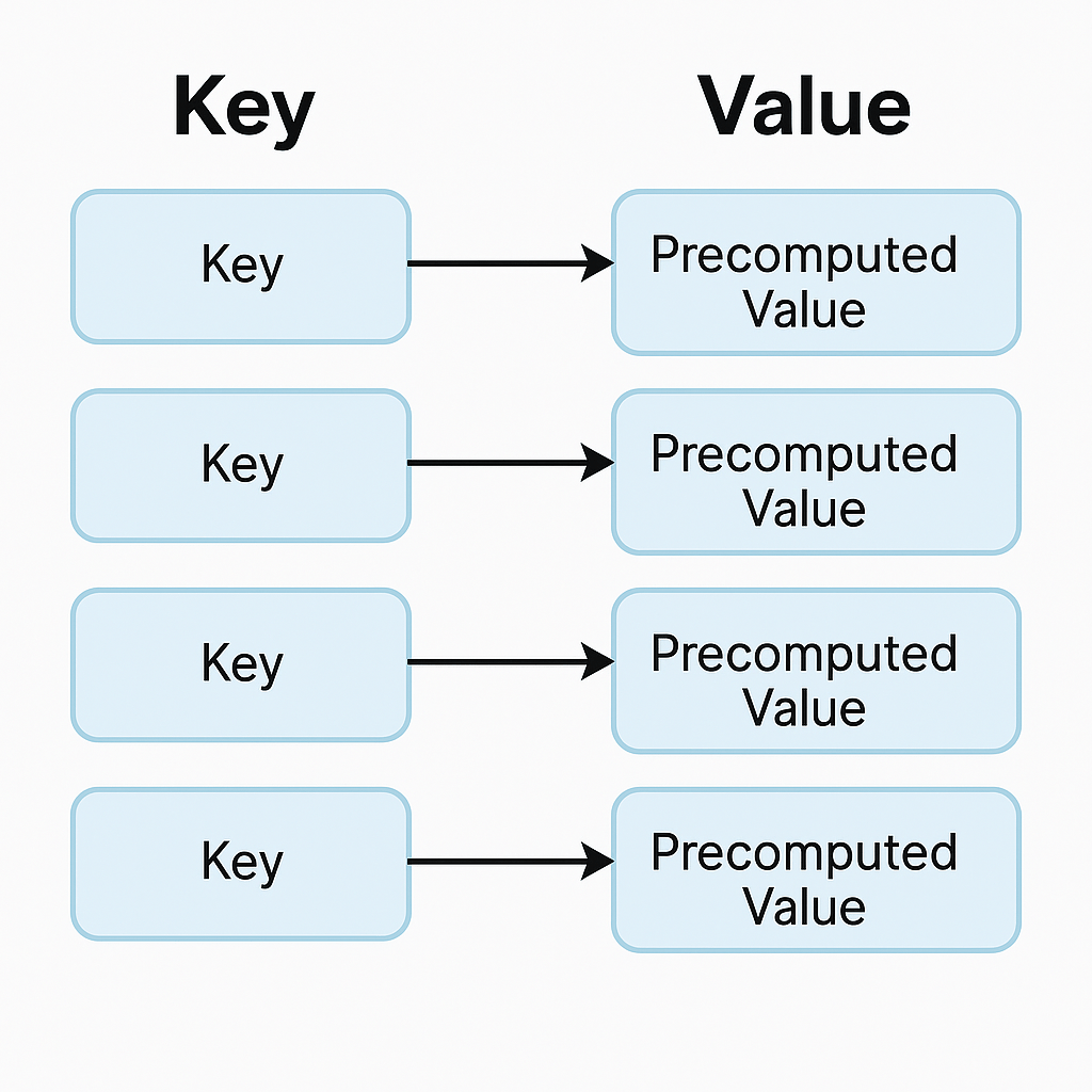
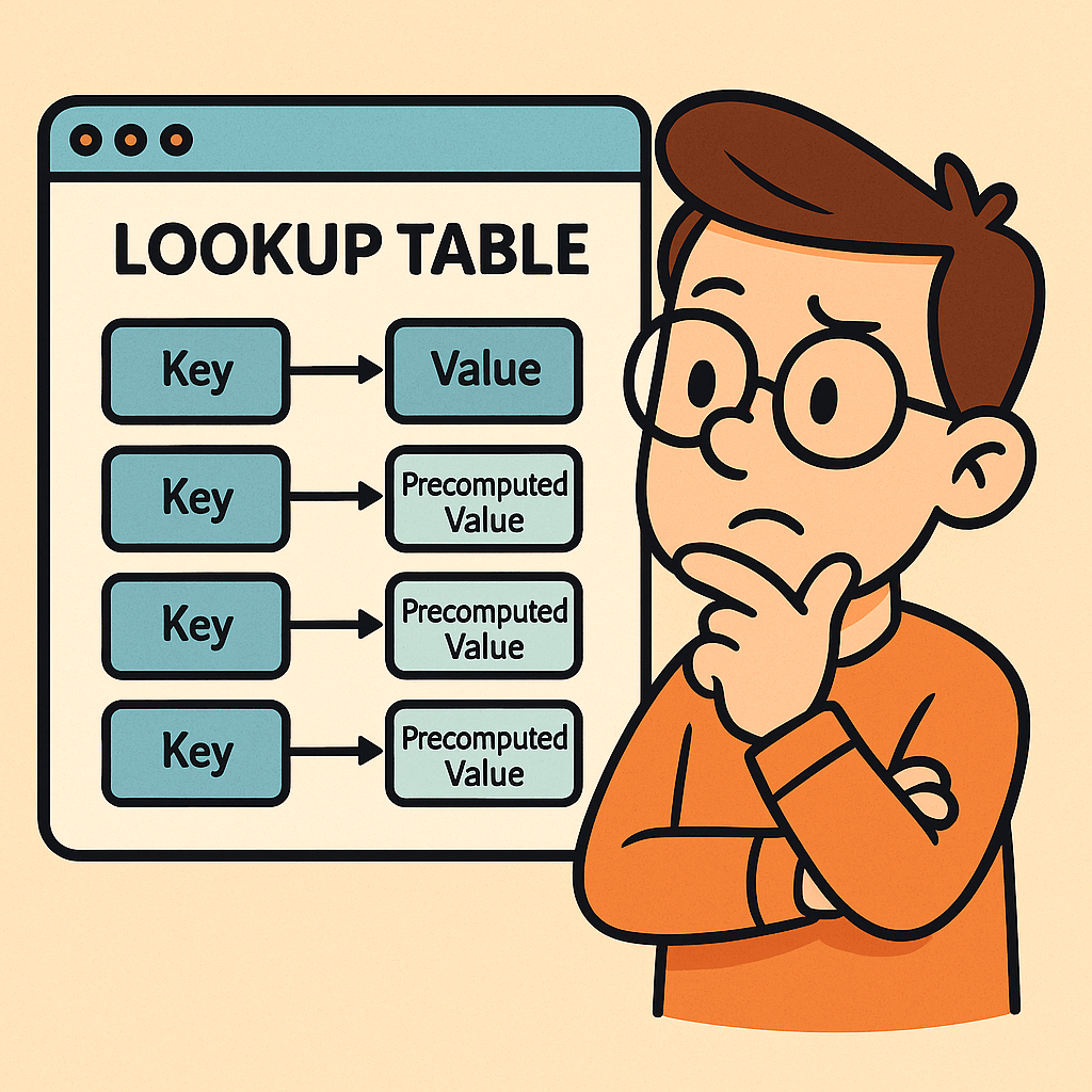
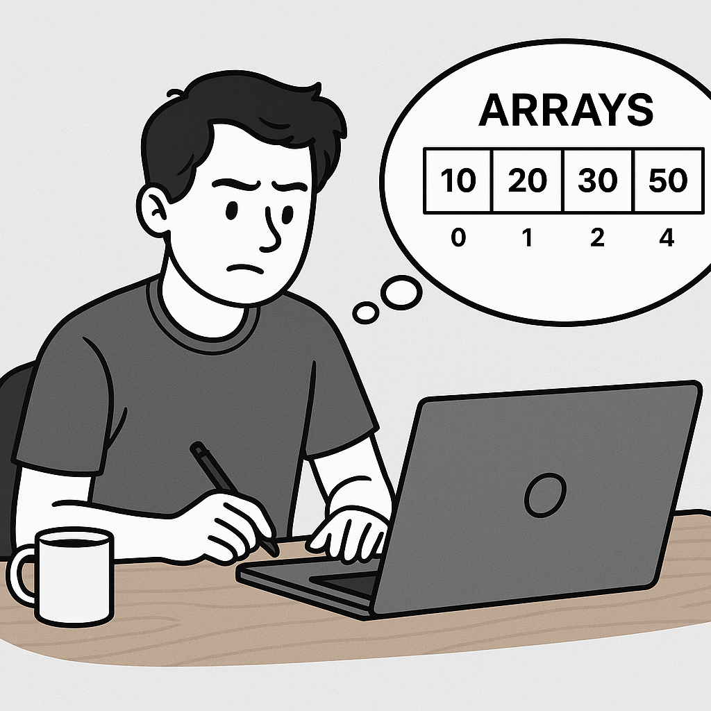
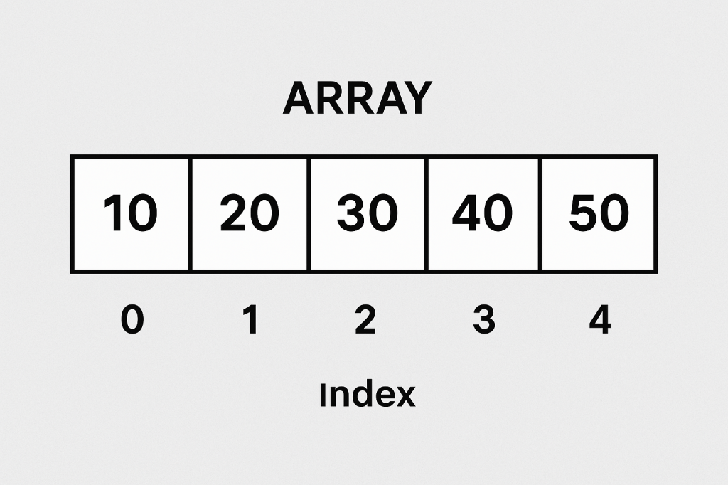
A lookup table (LUT) is a data structure, usually implemented as an array, hash map, or dictionary, that allows you to retrieve precomputed values based on an input key. Instead of recalculating a result every time it’s needed, the result is stored in advance and can be fetched in constant time.
Think of it as a cheat sheet for your program — instead of solving a problem from scratch, you look up the answer directly.
Why Do We Need Lookup Tables?
The main reason is performance optimization.
Some operations are expensive to compute repeatedly (e.g., mathematical calculations, data transformations, or lookups across large datasets). By precomputing the results and storing them in a lookup table, you trade memory for speed.
This is especially useful in systems where:
- The same operations occur frequently.
- Fast response time is critical.
- Memory is relatively cheaper compared to CPU cycles.
When Should We Use a Lookup Table?
You should consider using a lookup table when:
- Repetitive Computations: If the same calculation is performed multiple times.
- Finite Input Space: When the possible inputs are limited and known beforehand.
- Performance Bottlenecks: If profiling your code shows that repeated computation is slowing things down.
- Real-Time Systems: Games, embedded systems, and graphics rendering often rely heavily on lookup tables to meet strict performance requirements.
Real World Example
Imagine you are working with an image-processing program that frequently needs the sine of different angles. Computing sine using the Math.sin() function can be expensive if done millions of times per second.
Instead, you can precompute sine values for angles (say, every degree from 0° to 359°) and store them in a lookup table:
double[] sineTable = new double[360];
for (int i = 0; i < 360; i++) {
    sineTable[i] = Math.sin(Math.toRadians(i));
}

// Later usage
double value = sineTable[45]; // instantly gets sine(45°)
This way, you retrieve results instantly without recalculating.
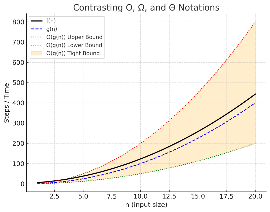
Time and Memory Complexities
Let’s analyze the common operations in a lookup table:
- Populating a Lookup Table:
- Time Complexity: O(n), where n is the number of entries you precompute.
- Memory Complexity: O(n), since you must store all values.
- Inserting an Element:
- Time Complexity: O(1) on average (e.g., in a hash map).
- Memory Complexity: O(1) additional space.
- Deleting an Element:
- Time Complexity: O(1) on average (e.g., marking or removing from hash table/array).
- Memory Complexity: O(1) freed space.
- Retrieving an Element (Lookup):
- Time Complexity: O(1) in most implementations (arrays, hash maps).
- This is the primary advantage of lookup tables.
Conclusion
A lookup table is a powerful optimization technique that replaces repetitive computation with direct retrieval. It shines when input values are limited and predictable, and when performance is critical. While it requires additional memory, the trade-off is often worth it for faster execution.
By understanding when and how to use lookup tables, you can significantly improve the performance of your applications.


Recent Comments