
What is Big-O notation?
Big-O notation describes how an algorithm’s running time or memory grows as the input size n gets large.
It gives an upper bound on growth—e.g., “this algorithm runs in O(n log n) time,” meaning its time won’t grow faster than some constant × n log n for large n. Big-O ignores machine details and constants so we can compare algorithms by their shape of growth, not their exact milliseconds on one computer.
Why Big-O matters
- Scalability: Today’s data set fits in RAM; tomorrow’s is 100× bigger. Big-O tells you who survives that jump.
- Design choices: Helps choose the right data structures/approaches (hash table vs. tree, brute-force vs. divide-and-conquer).
- Performance budgeting: If your endpoint must answer in 50 ms at 1M records, O(n²) is a red flag; O(log n) might be fine.
- Interview lingua franca: It’s the common vocabulary for discussing efficiency in interviews.
How to calculate Big-O
- Define the input size
n. (e.g., length of an array, number of nodes.) - Count dominant operations as a function of
n(comparisons, swaps, hash lookups, etc.). - Focus on worst-case unless stated otherwise (best/average can be different).
- Drop constants and lower-order terms.
3n² + 2n + 7→ O(n²). - Use composition rules:
- Sequential steps add:
O(f(n)) + O(g(n))→O(f(n) + g(n)), usually dominated by the larger term. - Loops multiply: a loop of
niterations doingO(g(n))work →O(n · g(n)). - Nested loops multiply their ranges: outer
n, innern→O(n²). - Divide-and-conquer often yields recurrences (e.g.,
T(n)=a·T(n/b)+O(n)) solved via the Master Theorem (e.g., mergesort → O(n log n)).
- Sequential steps add:
Step-by-step example: from counts to O(n²)
Goal: Compute the Big-O of this function.
def count_pairs(a):        # a has length n
    total = 0              # 1
    for i in range(len(a)):           # runs n times
        for j in range(i, len(a)):    # runs n - i times
            total += 1                 # 1 per inner iteration
    return total           # 1
Operation counts
- The inner statement
total += 1executes for each pair(i, j)with0 ≤ i ≤ j < n.
Total executions =n + (n-1) + (n-2) + … + 1 = n(n+1)/2. - Add a few constant-time lines (initialization/return). They don’t change the growth class.
Total time T(n) is proportional to n(n+1)/2.
Expand: T(n) = (n² + n)/2 = (1/2)n² + (1/2)n.
Drop constants and lower-order terms → O(n²).
Takeaway: Triangular-number style nested loops typically lead to O(n²).
(Bonus sanity check: If we changed the inner loop to a fixed 10 iterations, we’d get n*10 → O(n).)
Quick Reference: Common Big-O Complexities
- O(1) — constant time (hash lookup, array index)
- O(log n) — binary search, balanced BST operations
- O(n) — single pass, counting, hash-map inserts (amortized)
- O(n log n) — efficient sorts (mergesort, heapsort), many divide-and-conquer routines
- O(n²) — simple double loops (all pairs)
- O(2ⁿ), O(n!) — exhaustive search on subsets/permutations
Big-O growth graph
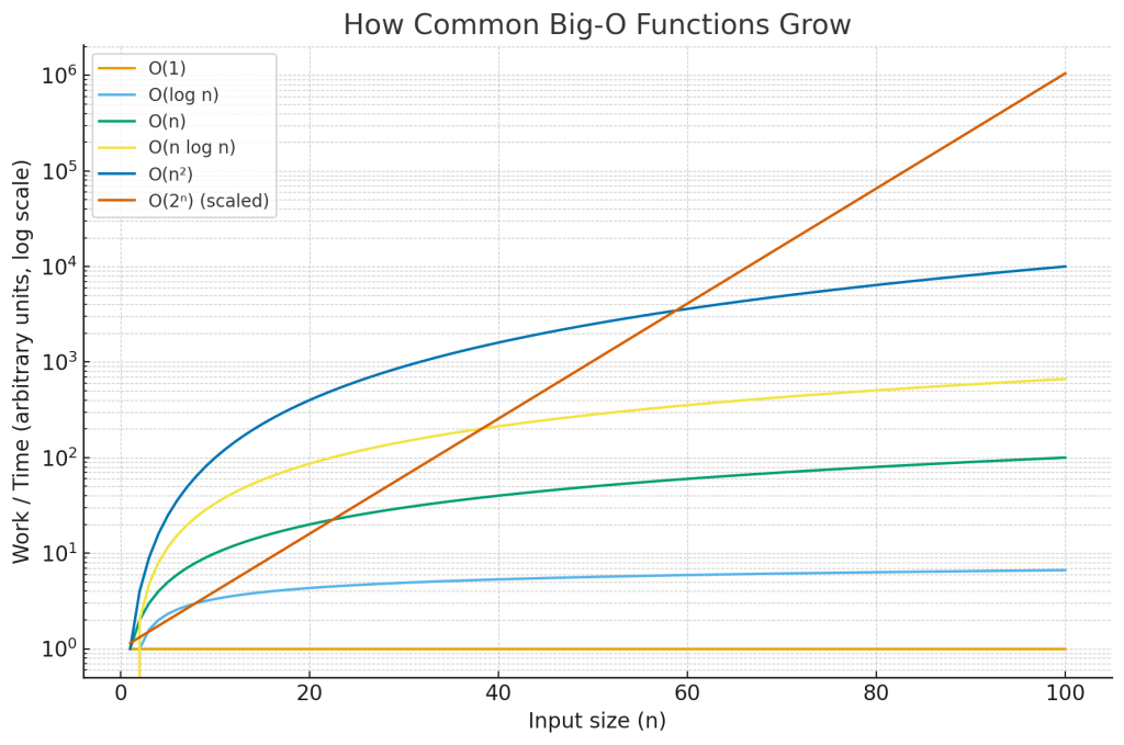
The chart above compares how common Big-O functions grow as n increases. The y-axis is logarithmic so you can see everything on one plot; on a normal (linear) axis, the exponential curve would shoot off the page and hide the differences among the slower-growing functions.
- Flat line (O(1)): work doesn’t change with input size.
- Slow curve (O(log n)): halves the problem each step—scales very well.
- Straight diagonal (O(n)): time grows linearly with input.
- Slightly steeper (O(n log n)): common for optimal comparison sorts.
- Parabola on linear axes (O(n²)): fine for small
n, painful past a point. - Explosive (O(2ⁿ)): only viable for tiny inputs or with heavy pruning/heuristics.

Recent Comments