Search

Software Engineer's Notes

Tag

programming

int vs Integer in Java: What They Are, Why Both Exist, and How to Choose

Quick Decision Guide

  • Use int for primitive number crunching, counters, loops, and performance-critical code.
  • Use Integer when you need null, work with collections/generics/Streams, use it as a map key, or interact with APIs that require objects.

What Are int and Integer?

  • int is a primitive 32-bit signed integer type.
    • Range: −2,147,483,648 to 2,147,483,647.
    • Stored directly on the stack or inside objects as a raw value.
  • Integer is the wrapper class for int (in java.lang).
    • An immutable object that contains an int value (or can be null).
    • Provides methods like compare, parseInt (static in Integer), etc.

Why Do We Have Two Types?

Java was designed with primitives for performance and memory efficiency. Later, Java introduced generics, Collections, and object-oriented APIs that need reference types. Wrapper classes (like Integer) bridge primitives and object APIs, enabling features primitives can’t provide (e.g., nullability, method parameters of type Object, use as generic type arguments).

Key Differences at a Glance

Aspectint (primitive)Integer (wrapper class)
NullabilityCannot be nullCan be null
Memory4 bytes for the valueObject header + 4 bytes value (+ padding)
PerformanceFast (no allocation)Slower (allocation, GC, boxing/unboxing)
Generics/CollectionsNot allowed as type parameterAllowed: List<Integer>
Default value (fields)0null
Equality== compares values== compares references; use .equals() for value
AutoboxingNot applicableWorks with int via autoboxing/unboxing
MethodsN/AUtility & instance methods (compareTo, hashCode, etc.)

Autoboxing & Unboxing (and the Gotchas)

Java will automatically convert between int and Integer:

Integer a = 5;    // autoboxing: int -> Integer
int b = a;        // unboxing: Integer -> int

Pitfall: Unboxing a null Integer throws NullPointerException.

Integer maybeNull = null;
int x = maybeNull; // NPE at runtime!

Tip: When a value can be absent, prefer OptionalInt/Optional<Integer> or check for null before unboxing.

Integer Caching (−128 to 127)

Integer.valueOf(int) caches values in [−128, 127]. This can make some small values appear identical by reference:

Integer x = 100;
Integer y = 100;
System.out.println(x == y);      // true (same cached object)
System.out.println(x.equals(y)); // true

Integer p = 1000;
Integer q = 1000;
System.out.println(p == q);      // false (different objects)
System.out.println(p.equals(q)); // true

Rule: Always use .equals() for value comparison with wrappers.

When to Use int

  • Counters, indices, arithmetic in tight loops.
  • Performance-critical code paths to avoid allocation/GC.
  • Fields that are always present (never absent) and don’t need object semantics.
  • Switch statements and bit-level operations.

Example:

int sum = 0;
for (int i = 0; i < nums.length; i++) {
  sum += nums[i];
}

When to Use Integer

  • Collections/Generics/Streams require reference types:
List<Integer> scores = List.of(10, 20, 30);

  • Nullable numeric fields (e.g., optional DB columns, partially populated DTOs).
  • Map keys or values where object semantics and equals/hashCode matter:
Map<Integer, String> userById = new HashMap<>();

  • APIs that expect Object or reflection/serialization frameworks.

Benefits of Each

Benefits of int

  • Speed & low memory footprint.
  • No NullPointerException from unboxing.
  • Straightforward arithmetic.

Benefits of Integer

  • Nullability to represent “unknown/missing”.
  • Works with Collections, Generics, Streams.
  • Provides utility methods and can be used in APIs requiring objects.
  • Immutability makes it safe as a map key.

When Not to Use Them

  • Avoid Integer in hot loops or large arrays where performance/memory is critical (boxing creates many objects).
    • Prefer int[] over List<Integer> when possible.
  • Avoid int when a value might be absent or needs to live in a collection or generic API.
  • Beware of unboxing nulls—if a value can be null, don’t immediately unbox to int.

Practical Patterns

1) DTO with Optional Field

class ProductDto {
  private Integer discountPercent; // can be null if no discount
  // getters/setters
}

2) Streams: Primitive vs Boxed

int sum = IntStream.of(1, 2, 3).sum();          // primitive stream: fast
int sum2 = List.of(1, 2, 3).stream()
                 .mapToInt(Integer::intValue)
                 .sum();                         // boxed -> primitive

3) Safe Handling of Nullable Integer

Integer maybe = fetchCount();           // might be null
int count = (maybe != null) ? maybe : 0; // avoid NPE

4) Overloads & Method Selection

If you provide both:

void setValue(int v) { /* ... */ }
void setValue(Integer v) { /* ... */ }

  • Passing a literal (setValue(5)) picks int.
  • Passing null only compiles for Integer (setValue(null)).

Common FAQs

Q: Why does List<int> not compile?
A: Generics require reference types; use List<Integer> or int[].

Q: Why does x == y sometimes work for small Integers?
A: Because of Integer caching (−128 to 127). Don’t rely on it—use .equals().

Q: I need performance but also collections—what can I do?
A: Use primitive arrays (int[]) or primitive streams (IntStream) to compute, then convert minimally when you must interact with object-based APIs.

Cheat Sheet

  • Performance: int > Integer
  • Nullability: Integer
  • Collections/Generics: Integer
  • Equality: int uses ==; Integer use .equals() for values
  • Hot loops / big data: prefer int / int[]
  • Optional numeric: Integer or OptionalInt (for primitives)

Mini Example: Mixing Both Correctly

class Scoreboard {
  private final Map<Integer, String> playerById = new HashMap<>(); // needs Integer
  private int totalScore = 0;                                      // fast primitive

  void addScore(int playerId, int score) {
    totalScore += score; // primitive math
    playerById.put(playerId, "Player-" + playerId);
  }

  Integer findPlayer(Integer playerId) {
    // Accepts null safely; returns null if absent
    return (playerId == null) ? null : playerId;
  }
}

Final Guidance

  • Default to int for computation and tight loops.
  • Choose Integer for nullability and object-centric APIs (Collections, Generics, frameworks).
  • Watch for NPE from unboxing and avoid boxing churn in performance-sensitive code.
  • Use .equals() for comparing Integer values; not ==.

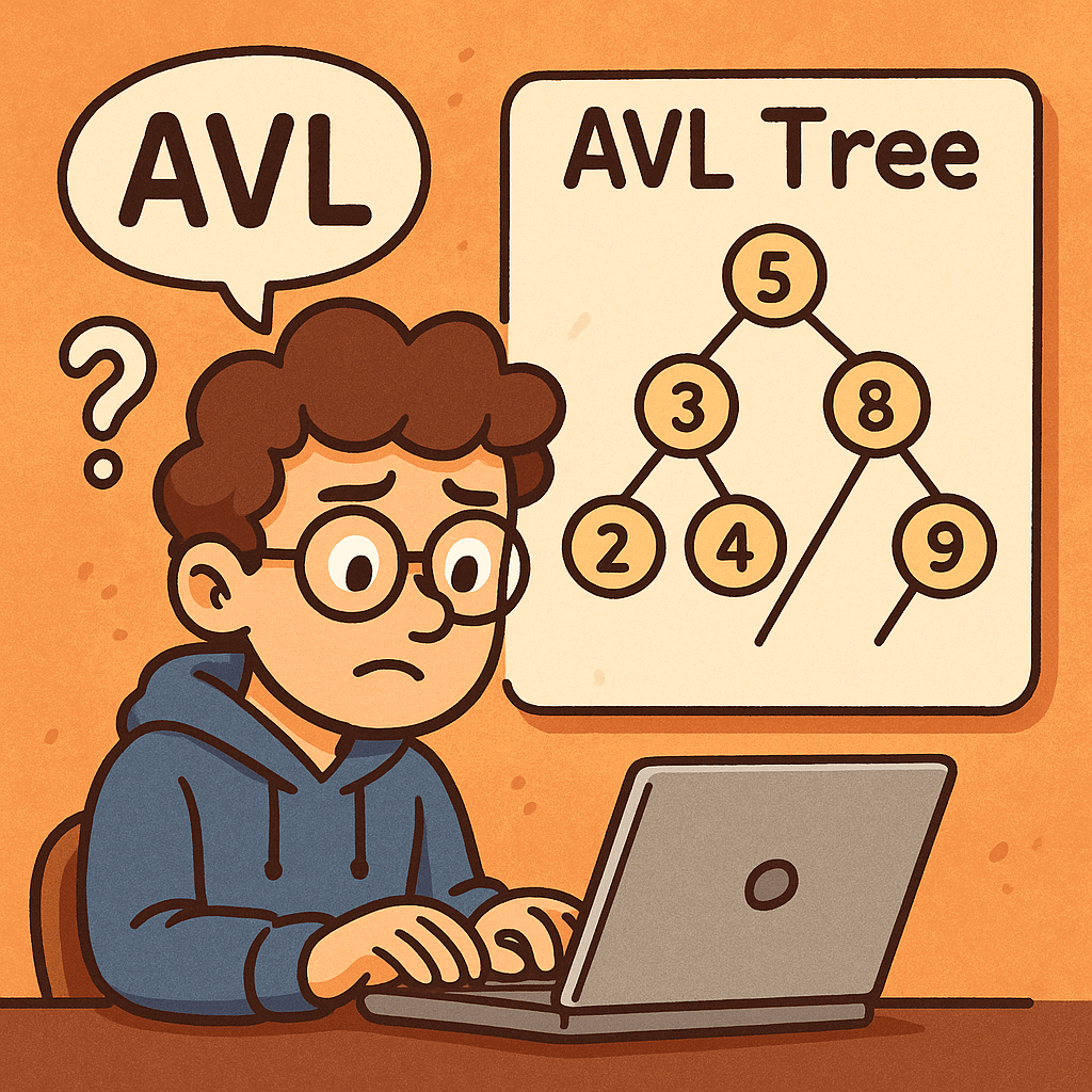
AVL Trees: A Practical Guide for Developers

What is an AVL Tree?

An AVL tree (named after Adelson-Velsky and Landis) is a self-balancing Binary Search Tree (BST).
For every node, the balance factor (height of left subtree − height of right subtree) is constrained to −1, 0, or +1. When inserts or deletes break this rule, the tree rotates (LL, RR, LR, RL cases) to restore balance—keeping the height O(log n).

Key idea: By preventing the tree from becoming skewed, every search, insert, and delete stays fast and predictable.

When Do We Need It?

Use an AVL tree when you need ordered data with consistently fast lookups and you can afford a bit of extra work during updates:

  • Read-heavy workloads where searches dominate (e.g., 90% reads / 10% writes)
  • Realtime ranking/leaderboards where items must stay sorted
  • In-memory indexes (e.g., IDs, timestamps) for low-latency search and range queries
  • Autocomplete / prefix sets (when implemented over keys that must remain sorted)

Real-World Example

Imagine a price alert service maintaining thousands of stock tickers in memory, keyed by last-trade time.

  • Every incoming request asks, “What changed most recently?” or “Find the first ticker after time T.”
  • With an AVL tree, search and successor/predecessor queries remain O(log n) even during volatile trading, while rotations keep the structure balanced despite frequent inserts/deletes.

Main Operations and Complexity

Operations

  • Search(k) – standard BST search
  • Insert(k, v) – BST insert, then rebalance with rotations (LL, RR, LR, RL)
  • Delete(k) – BST delete (may replace with predecessor/successor), then rebalance
  • Find min/max, predecessor/successor, range queries

Time Complexity

  • Search: O(log n)
  • Insert: O(log n) (includes at most a couple of rotations)
  • Delete: O(log n) (may trigger rotations)
  • Min/Max, predecessor/successor: O(log n)

Space Complexity

  • Space: O(n) for nodes
  • Per-node overhead: O(1) (store height or balance factor)

Advantages

  • Guaranteed O(log n) for lookup, insert, delete (tighter balance than many alternatives)
  • Predictable latency under worst-case patterns (no pathologically skewed trees)
  • Great for read-heavy or latency-sensitive workloads

Disadvantages

  • More rotations/updates than looser trees (e.g., Red-Black) → slightly slower writes
  • Implementation complexity (more cases to handle correctly)
  • Cache locality worse than B-trees on disk; not ideal for large on-disk indexes

Quick Note on Rotations

  • LL / RR: one single rotation fixes it
  • LR / RL: a double rotation (child then parent) fixes it
    Rotations are local (affect only a few nodes) and keep the BST order intact.

AVL vs. (Plain) Binary Tree — What’s the Difference?

Many say “binary tree” when they mean “binary search tree (BST).” A plain binary tree has no ordering or balancing guarantees.
An AVL is a BST + balance rule that keeps height logarithmic.

FeaturePlain Binary TreeUnbalanced BSTAVL (Self-Balancing BST)
Ordering of keysNot requiredIn-order (left < node < right)In-order (left < node < right)
Balancing ruleNoneNoneHeight difference per node ∈ {−1,0,+1}
Worst-case heightO(n)O(n) (e.g., sorted inserts)O(log n)
SearchO(n) worst-caseO(n) worst-caseO(log n)
Insert/DeleteO(1)–O(n)O(1)–O(n)O(log n) (with rotations)
Update overheadMinimalMinimalModerate (rotations & height updates)
Best forSimple trees/traversalsWhen input is random and smallRead-heavy, latency-sensitive, ordered data

When to Prefer AVL Over Other Trees

  • Choose AVL when you must keep lookups consistently fast and don’t mind extra work on writes.
  • Choose Red-Black Tree when write throughput is a bit more important than the absolute tightness of balance.
  • Choose B-tree/B+-tree for disk-backed or paged storage.

Minimal Insert (Pseudo-Java) for Intuition

class Node {
  int key, height;
  Node left, right;
}

int h(Node n){ return n==null?0:n.height; }
int bf(Node n){ return n==null?0:h(n.left)-h(n.right); }
void upd(Node n){ n.height = 1 + Math.max(h(n.left), h(n.right)); }

Node rotateRight(Node y){
  Node x = y.left, T2 = x.right;
  x.right = y; y.left = T2;
  upd(y); upd(x);
  return x;
}
Node rotateLeft(Node x){
  Node y = x.right, T2 = y.left;
  y.left = x; x.right = T2;
  upd(x); upd(y);
  return y;
}

Node insert(Node node, int key){
  if(node==null) return new Node(){ {this.key=key; this.height=1;} };
  if(key < node.key) node.left = insert(node.left, key);
  else if(key > node.key) node.right = insert(node.right, key);
  else return node; // no duplicates

  upd(node);
  int balance = bf(node);

  // LL
  if(balance > 1 && key < node.left.key) return rotateRight(node);
  // RR
  if(balance < -1 && key > node.right.key) return rotateLeft(node);
  // LR
  if(balance > 1 && key > node.left.key){ node.left = rotateLeft(node.left); return rotateRight(node); }
  // RL
  if(balance < -1 && key < node.right.key){ node.right = rotateRight(node.right); return rotateLeft(node); }

  return node;
}

Summary

  • AVL = BST + strict balanceheight O(log n)
  • Predictable performance for search/insert/delete: O(log n)
  • Best for read-heavy or latency-critical ordered data; costs a bit more on updates.
  • Compared to a plain binary tree or unbalanced BST, AVL avoids worst-case slowdowns by design.

Binary Trees: A Practical Guide for Developers

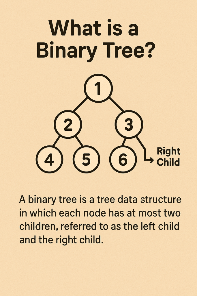
A binary tree is a hierarchical data structure where each node has at most two children. It’s great for ordered data, fast lookups/insertions (often near O(log n)), and in-order traversal. With balancing (AVL/Red-Black), performance becomes reliably logarithmic. Downsides include pointer overhead and potential O(n) worst-cases if unbalanced.

What Is a Binary Tree?

A binary tree is a collection of nodes where:

  • Each node stores a value.
  • Each node has up to two child references: left and right.
  • The top node is the root; leaf nodes have no children.

Common variants

  • Binary Search Tree (BST): Left subtree values < node < right subtree values (enables ordered operations).
  • Balanced BSTs: (e.g., AVL, Red-Black) keep height ≈ O(log n) for consistent performance.
  • Heap (Binary Heap): Complete tree with heap property (parent ≤/≥ children); optimized for min/max retrieval, not for sorted in-order traversals.
  • Full/Complete/Perfect Trees: Structural constraints that affect height and storage patterns.

Key terms

  • Height (h): Longest path from root to a leaf.
  • Depth: Distance from root to a node.
  • Subtree: A tree formed by a node and its descendants.

When Do We Need It?

Use a binary tree when you need:

  • Ordered data with frequent inserts/lookups (BSTs).
  • Sorted iteration via in-order traversal without extra sorting.
  • Priority access (heaps for schedulers, caches, and task queues).
  • Range queries (e.g., “all keys between A and M”) more naturally than in hash maps.
  • Memory-efficient dynamic structure that grows/shrinks without contiguous arrays.

Avoid it when:

  • You only need exact-key lookups with no ordering → Hash tables may be simpler/faster on average.
  • Data is largely sequential/indexedArrays/ArrayLists can be better.

Real-World Example

Autocomplete suggestions (by prefix):

  1. Store words in a BST keyed by the word itself (or a custom key like (prefix, word)).
  2. To suggest completions for prefix “em”, find the lower_bound (“em…”) node, then do in-order traversal while keys start with “em”.
  3. This provides sorted suggestions with efficient insertions as vocabulary evolves.
    (If extreme scale/branching is needed, a trie may be even better—but BSTs are a simple, familiar starting point.)

Another quick one: Task scheduling with a min-heap (a binary heap). The smallest deadline pops first in O(log n), ideal for job schedulers.

Main Operations & Complexity

On a (possibly unbalanced) Binary Search Tree

OperationAverage TimeWorst TimeSpace (extra)
Search (find key)O(log n)O(n)O(1) iterative; O(h) recursive
InsertO(log n)O(n)O(1) / O(h)
DeleteO(log n)O(n)O(1) / O(h)
In-order/Preorder/Postorder TraversalO(n)O(n)O(h)
Level-order (BFS)O(n)O(n)O(w) (w = max width)
  • n = number of nodes, h = height of the tree (worst n−1), w = max nodes at any level.
  • A balanced BST keeps h ≈ log₂n, making search/insert/delete reliably O(log n).

On a Binary Heap

OperationTime
Push/InsertO(log n)
Pop Min/MaxO(log n)
Peek Min/MaxO(1)
Build-heap (from array)O(n)

Space for the tree overall is O(n). Traversals use O(h) stack space recursively (or O(1) if done iteratively with your own stack/queue memory accounted as O(n) in BFS).

Core Operations Explained (BST)

  • Search: Compare key at node; go left if smaller, right if larger; stop when equal or null.
  • Insert: Search where the key would be; attach a new node there.
  • Delete:
    • Leaf: remove directly.
    • One child: bypass node (link parent → child).
    • Two children: replace value with in-order successor (smallest in right subtree), then delete that successor node.
  • Traversal:
    • In-order (LNR): yields keys in sorted order.
    • Preorder (NLR): useful for serialization/cloning.
    • Postorder (LRN): useful for deletions/freeing.

Advantages

  • Near-logarithmic performance for search/insert/delete with balancing.
  • Maintains order → easy sorted iteration and range queries.
  • Flexible structure → no need for contiguous memory; easy to grow/shrink.
  • Rich ecosystem → balanced variants (AVL, Red-Black), heaps, treaps, etc.

Disadvantages

  • Unbalanced worst-case can degrade to O(n) (e.g., inserting sorted data into a naive BST).
  • Pointer overhead per node (vs. compact arrays).
  • More complex deletes than arrays/lists or hash maps.
  • Cache-unfriendly due to pointer chasing (vs. contiguous arrays/heaps).

Practical Tips

  • If you need reliably fast operations, choose a self-balancing BST (AVL or Red-Black).
  • For priority queues, use a binary heap (typically array-backed, cache-friendlier).
  • For prefix/string-heavy tasks, consider a trie; for exact lookups without ordering, consider a hash map.
  • Watch out for recursion depth with very deep trees; consider iterative traversals.

Summary

Binary trees sit at the heart of many performant data structures. Use them when ordering matters, when you want predictable performance (with balancing), and when sorted traversals or range queries are common. Pick the specific variant—BST, balanced BST, or heap—based on your dominant operations.

Understanding Hash Tables: A Key Data Structure in Computer Science

When building efficient software, choosing the right data structure is critical. One of the most widely used and powerful data structures is the hash table. In this post, we’ll explore what a hash table is, why it’s useful, when to use it, and how it compares with a lookup table. We’ll also examine real-world examples and analyze its time and memory complexities.

What is a Hash Table?

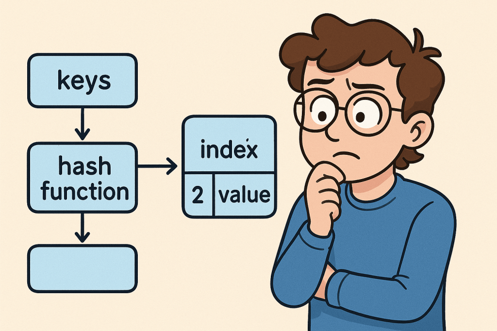
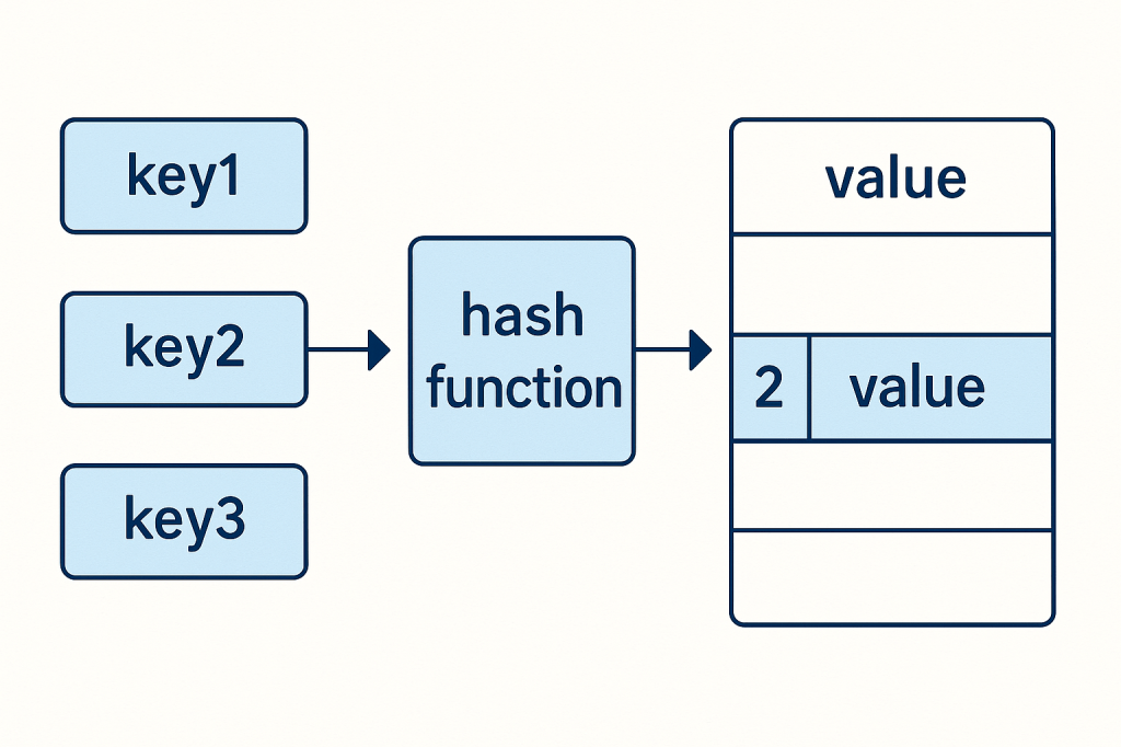
A hash table (also known as a hash map) is a data structure that stores key–value pairs.
It uses a hash function to convert keys into indexes, which point to where the corresponding value is stored in memory.

Think of it as a dictionary: you provide a word (the key), and the dictionary instantly gives you the definition (the value).

Why Do We Need a Hash Table?

Hash tables allow for fast lookups, insertions, and deletions. Unlike arrays or linked lists, where finding an item may take linear time, hash tables can usually perform these operations in constant time (O(1)).

This makes them essential for situations where quick access to data is needed.

When Should We Use a Hash Table?

You should consider using a hash table when:

  • You need fast lookups based on a unique key.
  • You are working with large datasets where performance matters.
  • You need to implement caches, dictionaries, or sets.
  • You want to avoid searching through long lists or arrays to find values.

Real-World Example

Imagine you are building a login system for a website.

  • You store usernames as keys.
  • You store hashed passwords as values.

When a user logs in, the system uses the username to quickly find the corresponding hashed password in the hash table and verify it.

Without a hash table, the system might need to search through a long list of users one by one, which would be very inefficient.

Time and Memory Complexities

Here’s a breakdown of the common operations in a hash table:

  • Inserting an element → Average: O(1), Worst-case: O(n) (when many collisions occur)
  • Deleting an element → Average: O(1), Worst-case: O(n)
  • Searching/Lookup → Average: O(1), Worst-case: O(n)
  • Memory Complexity → O(n), with additional overhead for handling collisions (like chaining or open addressing).

The efficiency depends on the quality of the hash function and how collisions are handled.

Is a Hash Table Different from a Lookup Table?

Yes, but they are related:

  • A lookup table is a precomputed array or mapping of inputs to outputs. It doesn’t necessarily require hashing — you might simply use an array index.
  • A hash table, on the other hand, uses hashing to calculate where a key should be stored, allowing flexibility for keys beyond just integers or array indexes.

In short:

  • Lookup Table = direct index mapping (fast but limited).
  • Hash Table = flexible key–value mapping using hashing.

Final Thoughts

Hash tables are one of the most versatile and powerful data structures in computer science. They allow developers to build high-performance applications, from caching systems to databases and authentication services.

Understanding when and how to use them can significantly improve the efficiency of your software.

Understanding Lookup Tables in Computer Science

When working with algorithms and data structures, efficiency often comes down to how quickly you can retrieve the information you need. One of the most powerful tools to achieve this is the Lookup Table. Let’s break down what it is, why we need it, when to use it, and the performance considerations behind it.

What is a Lookup Table?

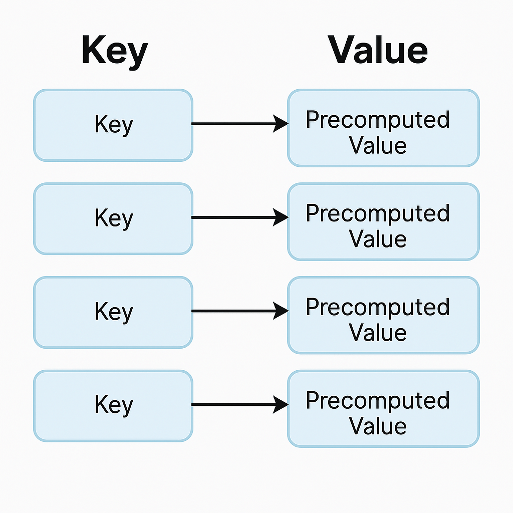
A lookup table (LUT) is a data structure, usually implemented as an array, hash map, or dictionary, that allows you to retrieve precomputed values based on an input key. Instead of recalculating a result every time it’s needed, the result is stored in advance and can be fetched in constant time.

Think of it as a cheat sheet for your program — instead of solving a problem from scratch, you look up the answer directly.

Why Do We Need Lookup Tables?

The main reason is performance optimization.
Some operations are expensive to compute repeatedly (e.g., mathematical calculations, data transformations, or lookups across large datasets). By precomputing the results and storing them in a lookup table, you trade memory for speed.

This is especially useful in systems where:

  • The same operations occur frequently.
  • Fast response time is critical.
  • Memory is relatively cheaper compared to CPU cycles.

When Should We Use a Lookup Table?

You should consider using a lookup table when:

  1. Repetitive Computations: If the same calculation is performed multiple times.
  2. Finite Input Space: When the possible inputs are limited and known beforehand.
  3. Performance Bottlenecks: If profiling your code shows that repeated computation is slowing things down.
  4. Real-Time Systems: Games, embedded systems, and graphics rendering often rely heavily on lookup tables to meet strict performance requirements.

Real World Example

Imagine you are working with an image-processing program that frequently needs the sine of different angles. Computing sine using the Math.sin() function can be expensive if done millions of times per second.

Instead, you can precompute sine values for angles (say, every degree from 0° to 359°) and store them in a lookup table:

double[] sineTable = new double[360];
for (int i = 0; i < 360; i++) {
    sineTable[i] = Math.sin(Math.toRadians(i));
}

// Later usage
double value = sineTable[45]; // instantly gets sine(45°)

This way, you retrieve results instantly without recalculating.

Time and Memory Complexities

Let’s analyze the common operations in a lookup table:

  • Populating a Lookup Table:
    • Time Complexity: O(n), where n is the number of entries you precompute.
    • Memory Complexity: O(n), since you must store all values.
  • Inserting an Element:
    • Time Complexity: O(1) on average (e.g., in a hash map).
    • Memory Complexity: O(1) additional space.
  • Deleting an Element:
    • Time Complexity: O(1) on average (e.g., marking or removing from hash table/array).
    • Memory Complexity: O(1) freed space.
  • Retrieving an Element (Lookup):
    • Time Complexity: O(1) in most implementations (arrays, hash maps).
    • This is the primary advantage of lookup tables.

Conclusion

A lookup table is a powerful optimization technique that replaces repetitive computation with direct retrieval. It shines when input values are limited and predictable, and when performance is critical. While it requires additional memory, the trade-off is often worth it for faster execution.

By understanding when and how to use lookup tables, you can significantly improve the performance of your applications.

Understanding Stacks in Data Structures

When learning about data structures, one of the simplest yet most powerful concepts is the stack. Just like its real-world counterpart—a stack of plates in your kitchen—this structure follows a very specific order for adding and removing items. Let’s dive deeper into what stacks are, why we need them, and where they shine in real-world applications.

What is a Stack?

A stack is a linear data structure that follows the LIFO (Last In, First Out) principle.

  • Last In → The last element added to the stack will be the first one removed.
  • First Out → The element added earliest will only be removed once everything added after it is removed.

Think of it as a pile of books—if you put a book on top, it’s the first one you’ll remove.

Stacks typically support two main operations:

  • Push → Add an element to the top.
  • Pop → Remove the element from the top.

Why Do We Need Stacks?

Stacks are crucial because they help us manage data in an order-dependent way. Their restricted operations make them predictable and efficient for solving problems where order of processing matters. Some common reasons we need stacks:

  • Managing function calls in programming (call stack).
  • Undo/redo functionality in applications.
  • Parsing expressions and checking balanced parentheses.
  • Backtracking algorithms (mazes, puzzles, etc.).

When Should We Use a Stack?

You should use a stack when:

  • You need to process elements in reverse order of their arrival.
  • You want a controlled way to temporarily store items.
  • You need fast insertion and removal at one end only.

If your use case involves removing items in the same order they were added, a queue (FIFO) might be more suitable.

A Real-World Example

Consider the browser back button.

  • Each time you visit a new page, the URL is pushed onto a stack.
  • When you press the back button, the last visited page is popped off, and the browser takes you to the previous one.

This is a perfect example of LIFO behavior in everyday life.

Time and Memory Complexities

Stacks are highly efficient since most operations occur at the top of the structure:

  • Pushing (insertion): O(1) – constant time.
  • Popping (deletion): O(1) – constant time.
  • Peeking (viewing top element): O(1) – constant time.
  • Memory complexity: O(n) – proportional to the number of elements stored.

This makes stacks a great fit when you need quick and predictable operations.

Final Thoughts

Stacks may sound simple, but they form the foundation of many critical systems in computer science. From managing program execution to enabling undo features in your favorite text editor, stacks are everywhere. Mastering them is a big step in becoming a stronger programmer.

Understanding ArrayLists in Programming

When working with data in programming, choosing the right data structure is critical. One of the most flexible and widely used data structures is the ArrayList. In this post, we’ll explore what ArrayLists are, why we need them, when to use them, and their time and memory complexities—with a real-world example to tie it all together.

What is an ArrayList?

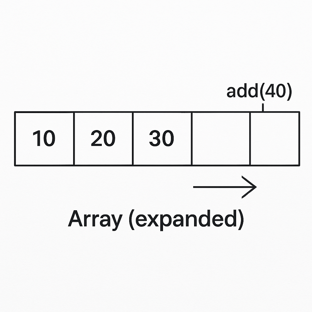
An ArrayList is a resizable array implementation provided in many programming languages (for example, java.util.ArrayList in Java or List<T> in C#). Unlike regular arrays that have a fixed size, ArrayLists can grow and shrink dynamically as elements are added or removed.

Think of an ArrayList as a dynamic array that provides built-in methods for managing data efficiently.

Why Do We Need an ArrayList?

Arrays are powerful, but they come with limitations:

  • Fixed size: once created, their size cannot change.
  • Manual resizing: you need to manage memory and copy elements if more space is needed.

ArrayLists solve these problems by:

  • Automatically resizing when more elements are added.
  • Providing handy methods like add(), remove(), contains(), and get() for easier management.
  • Allowing both random access (like arrays) and dynamic growth.

When Should We Use ArrayLists?

You should use an ArrayList when:

  • The number of elements in your collection is not known in advance.
  • You frequently need to add, remove, or search for elements.
  • You want random access to elements by index.
  • Performance is important, but you can tolerate occasional resizing overhead.

If you know the size in advance and memory efficiency is critical, a simple array might be better. But if flexibility matters, ArrayLists are the way to go.

Real-World Example of an ArrayList

Imagine you’re building a shopping cart in an e-commerce application.

  • Users can add items (products).
  • They can remove items at any time.
  • The cart needs to expand dynamically as users shop.

Here’s a Java snippet:

import java.util.ArrayList;

public class ShoppingCart {
    public static void main(String[] args) {
        ArrayList<String> cart = new ArrayList<>();

        // Adding items
        cart.add("Laptop");
        cart.add("Smartphone");
        cart.add("Headphones");

        System.out.println("Cart: " + cart);

        // Removing an item
        cart.remove("Smartphone");
        System.out.println("Cart after removal: " + cart);

        // Accessing an item
        System.out.println("First item: " + cart.get(0));
    }
}

Output:

Cart: [Laptop, Smartphone, Headphones]
Cart after removal: [Laptop, Headphones]
First item: Laptop

This example shows how ArrayLists let us manage collections dynamically without worrying about resizing manually.

Time and Memory Complexities

Understanding performance helps you make better design decisions. Here are the typical complexities for ArrayLists:

  • Populating (adding at the end):
    • Average case: O(1) (amortized constant time)
    • Worst case (when resizing happens): O(n)
  • Inserting an element at a specific index:
    • O(n) (because elements may need to shift)
  • Deleting an element:
    • O(n) (elements after the removed one shift left)
  • Accessing an element by index:
    • O(1) (direct access like an array)
  • Memory usage:
    • Slightly higher than arrays due to dynamic resizing overhead (extra space allocated to reduce frequent copying).

Conclusion

ArrayLists are one of the most useful data structures for everyday programming. They combine the fast access of arrays with the flexibility of dynamic collections. Whether you’re building a shopping cart, managing user sessions, or keeping track of tasks, ArrayLists provide a balance of performance and convenience.

Next time you’re faced with a growing list of elements, consider reaching for an ArrayList—it just might be the perfect fit.

Understanding Linked Lists: A Beginner’s Guide

When learning data structures, arrays are usually the first stop. But once you’ve mastered them, you’ll quickly discover a new structure that solves many of their limitations: the linked list.

In this blog, we’ll explore what a linked list is, why we need it, when to use it, provide a real-world example, and analyze the time and memory complexities of linked lists.

What is a Linked List?

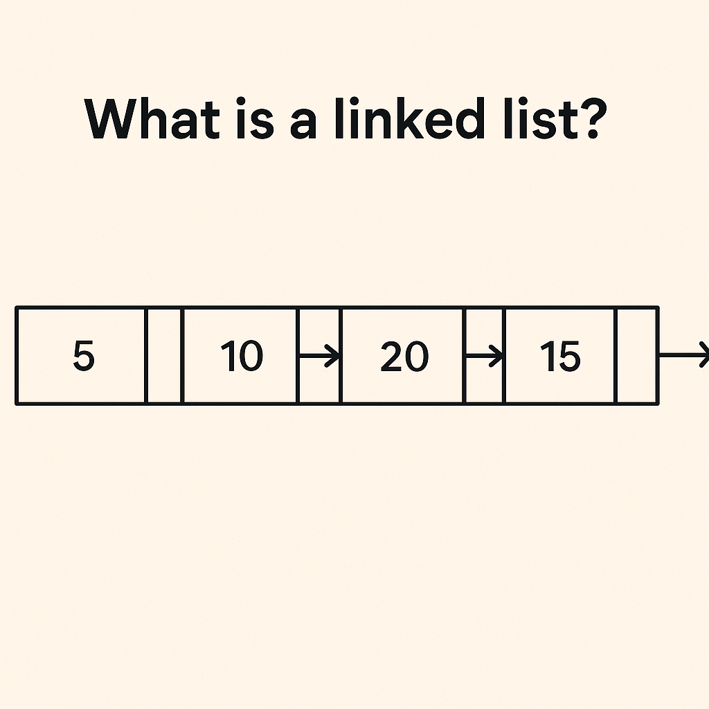
A linked list is a linear data structure where elements (called nodes) are stored in separate memory locations and connected using pointers (links).

Each node typically contains:

  • Data – the value you want to store
  • Pointer/Reference – an address pointing to the next node in the list

Unlike arrays, linked lists do not store elements in contiguous memory blocks.

Why Do We Need Linked Lists?

Arrays are simple and efficient for random access, but they come with drawbacks:

  • Fixed size (in most programming languages, arrays cannot grow dynamically without creating a new one)
  • Costly insertions and deletions (shifting elements takes time)

Linked lists solve these issues by:

  • Allowing dynamic memory allocation (they grow and shrink as needed)
  • Enabling fast insertions and deletions without shifting entire elements

When Should We Use Linked Lists?

You should consider linked lists when:

  • Memory is fragmented, and you can’t allocate a large contiguous block (required for arrays).
  • You expect frequent insertions and deletions, especially in the middle of the collection.
  • Random access is not a priority (linked lists are slower at accessing an element by index).

Real-World Example

Imagine a music playlist app.

  • Songs can be dynamically added or removed from the playlist.
  • You don’t know the total number of songs in advance.
  • You often skip to the next song (which is just following the pointer to the next node).

Here, a linked list structure is perfect because it supports efficient insertions, deletions, and sequential traversal.

Time & Memory Complexities

Here’s a quick overview of linked list operations:

OperationTime ComplexityExplanation
Populate (building a linked list of n elements)O(n)Each element needs to be inserted one by one
Insertion at headO(1)Just update the head pointer
Insertion at tailO(1) (if tail pointer is maintained) / O(n) (if not)Depends on whether you track the tail
Insertion in middleO(n)Need to traverse to the correct position
Deletion at headO(1)Update head pointer
Deletion at tailO(n)Need to traverse to the last element
Deletion in middleO(n)Traverse to find node, then remove
Access by indexO(n)Must traverse sequentially
Memory usageHigher than arraysEach node requires extra space for a pointer

Conclusion

Linked lists are powerful when dealing with dynamic data where frequent insertions and deletions occur. However, they trade off speed for random access and consume more memory due to pointers.

Understanding when to use arrays and when to use linked lists is a core skill every software engineer should master.

Understanding Arrays: A Complete Beginner’s Guide

Arrays are one of the most fundamental concepts in computer science and programming. Whether you are working with Java, Python, JavaScript, or PHP, arrays play a critical role in how data is stored and accessed. In this post, we’ll break down what arrays are, why they’re important, when to use them, and even analyze their performance.

What is an Array?

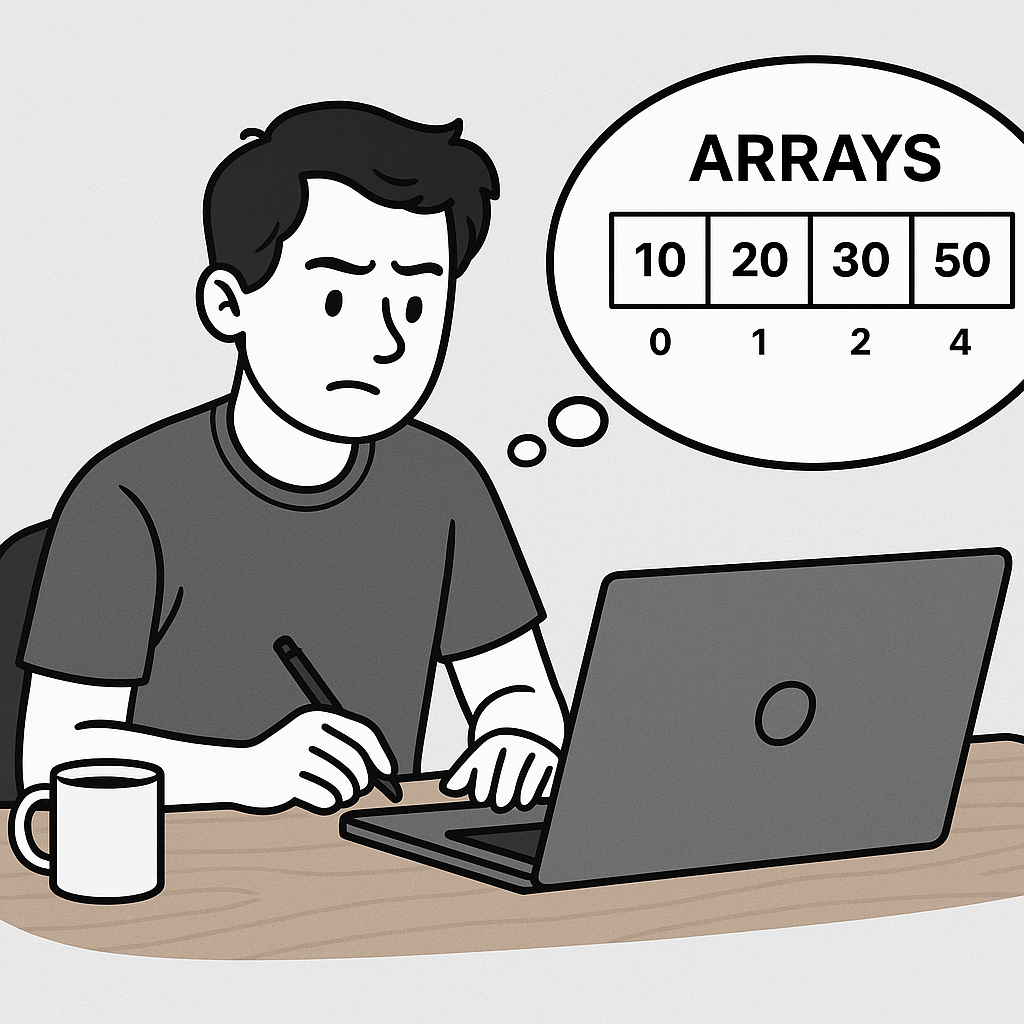
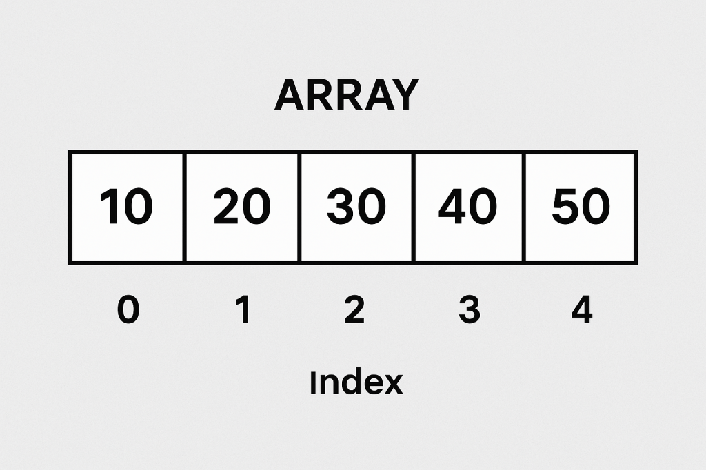
An array is a data structure that stores multiple values of the same type in a single variable. Instead of declaring multiple variables to hold related data, we can store them in an array and access them by their index (position).

Example in Java:

int numbers[] = {10, 20, 30, 40, 50};
System.out.println(numbers[2]); // prints 30

Here, numbers[2] refers to the third element in the array (since arrays are zero-indexed).

Why Do We Need Arrays?

Arrays solve the problem of managing large amounts of data efficiently. Without arrays, we would need to create separate variables for each value, which becomes unmanageable.

  • Organized data storage – Store related items together.
  • Fast access – Retrieve elements in constant time using an index.
  • Efficient looping – Easily iterate over items with for or while loops.

When Should We Use Arrays?

Use arrays when:

  • You know the fixed size of data in advance.
  • You want fast, random access to elements by index.
  • You want to perform repetitive operations on similar data types.

However, if the dataset size changes frequently (lots of insertions/deletions), arrays may not be the best choice. In such cases, dynamic structures like ArrayList in Java or List in Python are preferred.

Real-World Example of Arrays

Imagine a system that stores the grades of students in a class:

grades = [85, 90, 78, 92, 88]

# Find average grade
average = sum(grades) / len(grades)
print("Class Average:", average)

Instead of creating five different variables (grade1, grade2, grade3...), an array helps us store all grades in a single variable and compute results easily.

Time and Memory Complexity

Arrays are efficient but come with tradeoffs. Let’s look at their common operations:

OperationTime ComplexityMemory Impact
Access (arr[i])O(1)No extra memory
Update (arr[i] = x)O(1)No extra memory
Populate (initial fill)O(n)O(n) space
Insert (middle)O(n)May shift elements
Insert (end)O(1) (if space) / O(n) (resize)Extra memory if resized
Delete (middle)O(n)Shift elements left
Delete (end)O(1)No shift

Key takeaway: Arrays are excellent for fast access but not ideal for frequent insertions or deletions in the middle.

Conclusion

Arrays are the backbone of many algorithms and data structures. They provide an easy way to store, organize, and access data efficiently. While they shine in random access speed, they are less suitable when frequent modifications are needed. Understanding arrays is the first step toward mastering more advanced structures like linked lists, stacks, and queues.

Blog at WordPress.com.

Up ↑