Search

Software Engineer's Notes

Tag

coding

Understanding Dependency Injection in Software Development

Understanding Dependency Injection

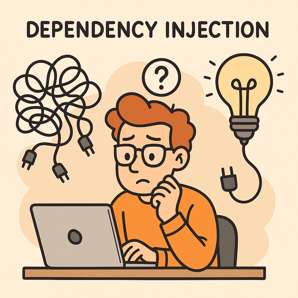
What is Dependency Injection?

Dependency Injection (DI) is a design pattern in software engineering where the dependencies of a class or module are provided from the outside, rather than being created internally. In simpler terms, instead of a class creating the objects it needs, those objects are “injected” into it. This approach decouples components, making them more flexible, testable, and maintainable.

For example, instead of a class instantiating a database connection itself, the connection object is passed to it. This allows the class to work with different types of databases without changing its internal logic.

A Brief History of Dependency Injection

The concept of Dependency Injection has its roots in the Inversion of Control (IoC) principle, which was popularized in the late 1990s and early 2000s. Martin Fowler formally introduced the term “Dependency Injection” in 2004, describing it as a way to implement IoC. Frameworks like Spring (Java) and later .NET Core made DI a first-class citizen in modern software development, encouraging developers to separate concerns and write loosely coupled code.

Main Components of Dependency Injection

Dependency Injection typically involves the following components:

  • Service (Dependency): The object that provides functionality (e.g., a database service, logging service).
  • Client (Dependent Class): The object that depends on the service to function.
  • Injector (Framework or Code): The mechanism responsible for providing the service to the client.

For example, in Java Spring:

  • The database service is the dependency.
  • The repository class is the client.
  • The Spring container is the injector that wires them together.

Why is Dependency Injection Important?

DI plays a crucial role in writing clean and maintainable code because:

  • It decouples the creation of objects from their usage.
  • It makes code more adaptable to change.
  • It enables easier testing by allowing dependencies to be replaced with mocks or stubs.
  • It reduces the “hardcoding” of configurations and promotes flexibility.

Benefits of Dependency Injection

  1. Loose Coupling: Clients are independent of specific implementations.
  2. Improved Testability: You can easily inject mock dependencies for unit testing.
  3. Reusability: Components can be reused in different contexts.
  4. Flexibility: Swap implementations without modifying the client.
  5. Cleaner Code: Reduces boilerplate code and centralizes dependency management.

When and How Should We Use Dependency Injection?

  • When to Use:
    • In applications that require flexibility and maintainability.
    • When components need to be tested in isolation.
    • In large systems where dependency management becomes complex.
  • How to Use:
    • Use frameworks like Spring (Java), Guice (Java), Dagger (Android), or ASP.NET Core built-in DI.
    • Apply DI principles when designing classes—focus on interfaces rather than concrete implementations.
    • Configure injectors (containers) to manage dependencies automatically.

Real World Examples of Dependency Injection

Spring Framework (Java):
A service class can be injected into a controller without explicitly creating an instance.

    @Service
    public class UserService {
        public String getUser() {
            return "Emre";
        }
    }
    
    @RestController
    public class UserController {
        private final UserService userService;
    
        @Autowired
        public UserController(UserService userService) {
            this.userService = userService;
        }
    
        @GetMapping("/user")
        public String getUser() {
            return userService.getUser();
        }
    }


    Conclusion

    Dependency Injection is more than just a pattern—it’s a fundamental approach to building flexible, testable, and maintainable software. By externalizing the responsibility of managing dependencies, developers can focus on writing cleaner code that adapts easily to change. Whether you’re building a small application or a large enterprise system, DI can simplify your architecture and improve long-term productivity.

    KISS Principle in Computer Science

    What is KISS principle?

    What is the KISS Principle?

    The KISS principle stands for “Keep It Simple, Stupid”, a design philosophy that emphasizes simplicity in systems, software, and problem-solving. Originally coined in the 1960s by the U.S. Navy, the principle highlights that most systems work best when they are kept simple rather than made unnecessarily complex.

    In computer science, KISS means writing code, designing architectures, and creating solutions that are straightforward, easy to understand, and easy to maintain. Simplicity reduces the likelihood of errors, speeds up development, and ensures long-term scalability.

    How Do You Apply the KISS Principle?

    Applying KISS requires conscious effort to avoid over-engineering or introducing complexity that is not needed. Some ways to apply it include:

    • Write readable code: Use clear naming conventions, simple logic, and avoid clever but confusing shortcuts.
    • Break problems into smaller pieces: Solve problems with modular, self-contained components.
    • Avoid unnecessary abstractions: Don’t add extra layers, classes, or patterns unless they solve a real need.
    • Leverage existing solutions: Use built-in language features or libraries rather than reinventing the wheel.
    • Document simply: Ensure documentation is concise and easy to follow.

    Benefits of the KISS Principle

    Keeping things simple offers multiple advantages:

    1. Maintainability – Simple systems are easier to maintain and update over time.
    2. Readability – Developers can quickly understand the logic without deep onboarding.
    3. Fewer bugs – Simplicity reduces the risk of introducing hidden issues.
    4. Faster development – Less complexity means faster coding, testing, and deployment.
    5. Better collaboration – Teams can work more effectively on systems that are easier to grasp.

    Main Considerations When Using KISS

    While simplicity is powerful, there are important considerations:

    • Balance with functionality: Simplicity should not come at the cost of missing essential features.
    • Avoid oversimplification: Stripping away too much may lead to fragile designs.
    • Think ahead, but not too far: Plan for scalability, but don’t build for problems that don’t exist yet.
    • Consistency matters: Simplicity is most effective when applied consistently across the entire codebase.

    Real-World Examples of KISS

    1. Unix Philosophy – Each tool does one thing well (e.g., grep, ls, cat). Instead of one complex tool, simple utilities are combined for powerful results.
    2. Hello World programs – A minimal program to test environments. It demonstrates clarity without unnecessary detail.
    3. RESTful APIs – Designed with simple, stateless principles that are easier to understand and scale compared to overly complex RPC systems.
    4. Version Control (Git) – Core commands like commit, push, and pull follow simple workflows. Advanced features exist, but the basics are simple and intuitive.

    Applying KISS in Software Development Processes

    Here are practical ways to embed KISS into your workflow:

    • Code reviews: Encourage reviewers to question unnecessary complexity.
    • Agile and iterative development: Build simple versions first (MVPs) and expand only if needed.
    • Design discussions: Ask, “Can this be made simpler?” before finalizing architectures.
    • Testing strategies: Simple unit tests are often more reliable than over-engineered test suites.
    • Refactoring sessions: Regularly revisit old code to simplify it as the system grows.

    Conclusion

    The KISS principle is a timeless guide for software engineers: simplicity is the key to robustness, maintainability, and efficiency. By applying it consistently, teams can build systems that last longer, are easier to maintain, and deliver more value with fewer headaches.

    Code Review in Software Development

    Learning code review

    What is a Code Review?

    A code review is the process of systematically examining source code written by a developer to identify mistakes, improve quality, and ensure adherence to coding standards. It is a peer-based activity where one or more team members review the code before it is merged into the main codebase.

    History of Code Review

    The concept of code review dates back to the early days of software engineering in the 1970s, when formal inspections were introduced by Michael Fagan at IBM. These inspections were strict, document-driven, and involved structured meetings. Over time, the practice evolved into more lightweight and flexible processes, especially with the rise of Agile and open-source development, where code review became a standard part of daily workflows.

    Importance of Code Review

    Code reviews are critical in modern software development. They:

    • Improve code quality and maintainability
    • Detect bugs early in the development cycle
    • Facilitate knowledge sharing among developers
    • Encourage collaboration and collective ownership of the code
    • Enforce coding standards and best practices

    Components of a Code Review

    A successful code review process usually involves:

    • Author: The developer who wrote the code.
    • Reviewers: Team members who evaluate the code.
    • Tools: Platforms such as GitHub, GitLab, Bitbucket, or specialized review tools.
    • Guidelines: Coding standards, project-specific conventions, and review checklists.
    • Feedback: Constructive comments, suggestions, and clarifications.

    How to Perform a Code Review

    • Start by understanding the purpose of the code changes.
    • Review smaller code changes instead of very large pull requests.
    • Check for correctness, readability, performance, and security.
    • Ensure the code follows style guides and project conventions.
    • Provide clear, respectful, and actionable feedback.
    • Encourage discussion instead of one-sided judgment.

    Is There a Formal Process?

    Yes, organizations often define formal processes for code reviews. A typical process may include:

    1. Developer submits code changes (pull request or merge request).
    2. Automated tests and linters run first.
    3. One or more reviewers analyze the code and leave comments.
    4. The author addresses feedback and makes changes.
    5. Reviewers approve the changes.
    6. Code is merged into the main branch.

    Some teams also use pair programming or walkthroughs as part of the process.

    Important Details to Pay Attention To

    Reviewers should pay attention to:

    • Logic and correctness of the code
    • Security vulnerabilities
    • Performance implications
    • Readability and maintainability
    • Compliance with coding standards
    • Proper documentation and comments

    While it’s important to catch issues, reviewers should avoid nitpicking too much on trivial details unless they affect the project long-term.

    How Much Time Should We Spend?

    Research suggests that effective code reviews should be 30 to 60 minutes per session, focusing on chunks of code not exceeding 400 lines at a time. Longer reviews often reduce effectiveness due to reviewer fatigue. The key is consistency—review regularly, not occasionally.

    Applying Code Review in Current Projects

    To integrate code reviews into your development process:

    • Use pull requests as the entry point for reviews.
    • Automate tests to catch basic issues before review.
    • Define clear review guidelines for your team.
    • Encourage collaborative discussions.
    • Use tools like GitHub, GitLab, or Bitbucket that integrate seamlessly with workflows.
    • Monitor review metrics (time spent, defects found, review coverage) to improve efficiency.

    String vs StringBuilder vs StringBuffer in Java

    String vs StringBuilder vs StringBuffer in Java

    Why Are There Three Similar Types?

    Java offers three string-related types to balance readability, safety, and performance:

    • String is simple and safe because it’s immutable.
    • StringBuilder is fast for single-threaded, heavy concatenation.
    • StringBuffer is like StringBuilder but synchronized for thread safety.

    Immutability (String) prevents accidental changes and enables pooling/caching. Mutability (StringBuilder/StringBuffer) avoids creating many temporary objects during repeated modifications.

    What Are They?

    String (Immutable, Thread-Safe by Design)

    • Once created, its content never changes.
    • Any “change” (e.g., concatenation) returns a new String.
    • String literals are stored in the string pool for memory efficiency.
    • Great for constants, keys, logging messages that don’t change, and APIs that return stable values.

    StringBuilder (Mutable, Not Synchronized)

    • Designed for fast, frequent modifications (append, insert, delete) in a single thread.
    • No synchronization overhead → typically the fastest way to build strings dynamically.

    StringBuffer (Mutable, Synchronized)

    • Like StringBuilder but synchronized methods for thread safety if the same builder is shared across threads.
    • Synchronization adds overhead, so it’s slower than StringBuilder in single-threaded code.

    Key Differences at a Glance

    Mutability

    • String: Immutable
    • StringBuilder: Mutable
    • StringBuffer: Mutable

    Thread Safety

    • String: Safe to share (cannot change)
    • StringBuilder: Not thread-safe
    • StringBuffer: Thread-safe (synchronized)

    Performance (Typical)

    • String: Fine for few ops; costly in large loops with + or +=
    • StringBuilder: Fastest for many concatenations in one thread
    • StringBuffer: Slower than StringBuilder due to synchronization

    Common APIs

    • String: rich APIs (substring, replace, split, equals, hashCode, compareTo)
    • StringBuilder/StringBuffer: builder-style APIs (append, insert, delete, reverse, setCharAt), then toString()

    How Do I Choose?

    Quick Decision Guide

    • Need a constant or rarely change the text? Use String.
    • Building text in a loop or via many appends in one thread? Use StringBuilder.
    • Building text shared across threads without external locks? Use StringBuffer (or prefer StringBuilder with your own synchronization strategy if you control access).

    Rule of Thumb

    • Use String by default for readability and safety.
    • Switch to StringBuilder when performance matters during repeated concatenations.
    • Use StringBuffer only when you truly need shared mutation across threads.

    Practical Examples

    Example 1: Costly Loop with String

    String s = "";
    for (int i = 0; i < 10000; i++) {
        s += i; // creates many temporary objects → avoid
    }


    Example 2: Efficient Loop with StringBuilder

    StringBuilder sb = new StringBuilder(10000); // optional capacity hint
    for (int i = 0; i < 10000; i++) {
        sb.append(i);
    }
    String s = sb.toString();


    Example 3: When StringBuffer Makes Sense

    // Only if 'shared' is truly accessed by multiple threads concurrently.
    StringBuffer shared = new StringBuffer();
    Runnable task = () -> {
        for (int i = 0; i < 1000; i++) {
            shared.append(i).append(",");
        }
    };


    Benefits of Each

    String

    • Simplicity and clarity
    • Inherent thread safety via immutability
    • Works well with string pooling (memory optimization)
    • Safe as map keys and for caching

    StringBuilder

    • Best performance for intensive concatenation
    • Low GC pressure versus many temporary Strings
    • Fluent, builder-style API

    StringBuffer

    • Built-in thread safety without external locks
    • Drop-in API similarity to StringBuilder

    When to Use Them (and When Not To)

    Use String When

    • Defining constants and literals
    • Passing values across layers/APIs
    • Storing keys in collections (immutability prevents surprises)

    Avoid String When

    • You’re repeatedly concatenating in loops (prefer StringBuilder)

    Use StringBuilder When

    • Building JSON, CSV, logs, or messages in loops
    • Formatting output dynamically in a single thread

    Avoid StringBuilder When

    • The builder is accessed by multiple threads simultaneously (unless you guard it externally)

    Use StringBuffer When

    • Multiple threads must mutate the same buffer at the same time and you can’t refactor for confinement

    Avoid StringBuffer When

    • You’re single-threaded or can confine builders per thread (prefer StringBuilder for speed)

    Additional Tips

    About the + Operator

    • In a single expression, the compiler typically uses an internal StringBuilder.
    • In loops, += often creates many intermediate objects. Prefer an explicit StringBuilder.

    Capacity Planning

    • Builders start with a default capacity and grow (usually doubling plus a small constant).
    • If you can estimate size, call new StringBuilder(expectedLength) or ensureCapacity to reduce reallocations.

    Interoperability

    • Convert builders to String with toString().
    • For equality checks, compare String values, not builders.

    Summary

    • String: Immutable, simple, safe → use by default for stable text.
    • StringBuilder: Mutable, fastest for repeated concatenations in one thread.
    • StringBuffer: Mutable, synchronized for shared multi-threaded mutation—use only when you truly need it.

    With these guidelines, choose the simplest type that meets your thread-safety and performance needs, and only optimize to builders when profiling or repeated concatenation calls for it.

    Understanding Queues in Computer Science

    Learning queue

    What is a Queue?

    what is queue

    A queue is a fundamental data structure in computer science that follows the FIFO (First In, First Out) principle. This means the first element inserted into the queue will be the first one removed. You can imagine it like a line at a supermarket: the first person who gets in line is the first to be served.

    Queues are widely used in software development for managing data in an ordered and controlled way.

    Why Do We Need Queues?

    Queues are important because they:

    • Maintain order of processing.
    • Prevent loss of data by ensuring all elements are handled in sequence.
    • Support asynchronous operations, such as task scheduling or handling requests.
    • Provide a reliable way to manage resources where multiple tasks compete for limited capacity (e.g., printers, processors).

    When Should We Use a Queue?

    You should consider using a queue when:

    • You need to process tasks in the order they arrive (job scheduling, message passing).
    • You need a buffer to handle producer-consumer problems (like streaming data).
    • You need fair resource sharing (CPU time slicing, printer spooling).
    • You’re managing asynchronous workflows, where events need to be handled one by one.

    Real World Example

    A classic example is a print queue.
    When multiple users send documents to a printer, the printer cannot handle them all at once. Instead, documents are placed into a queue. The printer processes the first document added, then moves on to the next, ensuring fairness and order.

    Another example is customer service call centers: calls are placed in a queue and answered in the order they arrive.

    Time and Memory Complexities

    Here’s a breakdown of queue operations:

    • Enqueue (Insert an element): O(1)
      Adding an element at the rear of the queue takes constant time.
    • Dequeue (Delete an element): O(1)
      Removing an element from the front of the queue also takes constant time.
    • Peek (Access the first element without removing it): O(1)
    • Memory Complexity: O(n)
      where n is the number of elements currently stored in the queue.

    Queues are efficient because insertion and deletion do not require shifting elements (unlike arrays).

    Conclusion

    Queues are simple yet powerful data structures that help maintain order and efficiency in programming. By applying the FIFO principle, they ensure fairness and predictable behavior in real-world applications such as scheduling, buffering, and resource management.

    Mastering queues is essential for every software engineer, as they are a cornerstone of many algorithms and system designs.

    Binary Search Trees (BST): A Practical Guide for Developers

    Learning Binary Search Tree

    A Binary Search Tree (BST) stores keys in sorted order so you can search, insert, and delete efficiently—typically in O(log n) time—if the tree stays balanced. It’s great when you need ordered data + fast lookups, but you must guard against becoming skewed (which degrades to O(n)).

    What is a Binary Search Tree?

    What is a Binary Search Tree?

    A Binary Search Tree (BST) is a binary tree where each node holds a key (and usually a value) and satisfies the BST property:

    • All keys in the left subtree are less than the node’s key.
    • All keys in the right subtree are greater than the node’s key.
    • This property holds recursively for every node.

    Because the keys are kept in sorted order, BSTs support ordered operations such as range queries and in-order traversal (which yields sorted output).

    When Do We Need a BST?

    Use a BST when you need both:

    1. Fast lookups/updates (ideally ~O(log n)), and
    2. Ordering-aware queries, like:
      • “Give me all keys between A and M.”
      • “What’s the next larger (successor) or next smaller (predecessor) key?”
      • “Iterate results in sorted order.”

    Common cases:

    • In-memory indexes (e.g., sorted maps/dictionaries).
    • Implementing priority features with order-aware operations (though heaps are better for pure min/max).
    • Autocomplete / prefix features (often with tries for strings, but BSTs work when comparing whole keys).
    • Scheduling or event timelines where you frequently need “next event after time T.”

    If you only need existence lookups without ordering, a hash table might be simpler and faster on average.

    Real-World Example

    E-commerce product catalog: Keep products keyed by productId or price.

    • Search a product quickly by ID.
    • List products in a price range (e.g., $25–$50) with an in-order traversal constrained to that range.
    • Find the next higher-priced product (successor) for upsell suggestions.

    Balanced BSTs (like AVL or Red-Black Trees) power the ordered collections in many standard libraries (e.g., TreeMap in Java, std::map in C++).

    Main Operations

    • Search(key): Compare key at node, go left if smaller, right if larger, stop when found or null.
    • Insert(key, value): Standard BST insert followed by optional rebalancing (in self-balancing variants).
    • Delete(key): Three cases
      1. Node has no child → remove it.
      2. Node has one child → replace node with its child.
      3. Node has two children → replace with in-order successor (smallest in right subtree) or predecessor, then delete that successor/predecessor node.
    • Traversal:
      • In-order → sorted order.
      • Pre-order/Post-order → useful for copying/deletion tasks.
    • Min/Max: Follow left/right pointers to extremes.
    • Successor/Predecessor: Use right/left subtree, or walk up via parent pointers if available.

    Time & Space Complexity

    OperationAverage (Balanced)Worst Case (Skewed)
    SearchO(log n)O(n)
    InsertO(log n)O(n)
    DeleteO(log n)O(n)
    Find min/max, successor/predecessorO(log n)O(n)
    Space (n nodes)O(n)O(n)

    In practice, self-balancing BSTs (AVL, Red-Black) keep height ≈ O(log n), ensuring predictable performance.

    Advantages

    • Maintains order: Easy to output or traverse in sorted order.
    • Efficient range queries: Retrieve keys within [L, R] without scanning everything.
    • Deterministic memory: Pointer-based structure with O(n) space.
    • Extensible: Augment nodes with extra data (e.g., subtree size for order statistics, sums for range aggregates).

    Disadvantages

    • Can degrade to O(n) if unbalanced (e.g., inserting already-sorted keys into a naive BST).
    • More complex deletions compared to hash tables or arrays.
    • Higher constant factors than hash tables for pure key→value lookups (when ordering isn’t needed).
    • Implementation complexity increases with self-balancing (AVL/Red-Black rotations, color/height tracking).

    BST vs. Alternatives (Quick Compare)

    • BST vs. Hash Table
      • BST: Ordered, range queries, successor/predecessor → Yes.
      • Hash: Average O(1) lookups, no order → great for pure key lookups.
    • BST vs. Array
      • BST: Fast inserts/deletes (O(log n) balanced) and maintains order.
      • Sorted array: Fast binary search (O(log n)), but inserts/deletes O(n).
    • BST vs. Heap
      • BST: Get any key, do range queries, get successor/predecessor.
      • Heap: Fastest min/max access, but no ordered iteration.

    Practical Tips & Pitfalls

    • Prefer self-balancing variants (e.g., AVL for tighter balance, Red-Black for simpler updates) in production.
    • To avoid skew, shuffle inputs or insert in mixed order if you must use a basic BST.
    • For heavy range queries, consider augmented BSTs (store subtree counts/sums) or B-trees for disk-based indices.
    • Use in-order traversal to stream results in sorted order without extra sorting cost.

    Summary

    A Binary Search Tree is a powerful, order-preserving data structure. Choose it when you need fast queries and ordering semantics—especially with self-balancing variants to maintain consistent O(log n) operations. If you don’t need order, a hash table is often simpler and faster; if you need just min/max, a heap may suffice.

    OptionalInt vs Optional in Java: When to Use Which (and Why)

    If you’ve worked with Java’s Optional<T>, you’ve probably also seen OptionalInt, OptionalLong, and OptionalDouble. Why does Java have both Optional<Integer> and OptionalInt? Which should you choose—and when?

    This guide breaks it down with clear examples and a simple decision checklist.

    • Optional<Integer> is the generic Optional for reference types. It’s flexible, works everywhere generics are needed, but boxes the int (adds memory & CPU overhead).
    • OptionalInt is a primitive specialization for int. It avoids boxing, is faster and lighter, and integrates nicely with IntStream, but is less flexible (no generics, fewer methods).

    Use OptionalInt inside performance-sensitive code and with primitive streams; use Optional<Integer> when APIs require Optional<T> or you need a uniform type.

    What Are They?

    Optional<Integer>

    A container that may or may not hold an Integer value:

    Optional<Integer> maybeCount = Optional.of(42);     // present
    Optional<Integer> emptyCount = Optional.empty();    // absent


    OptionalInt

    A container specialized for the primitive int:

    OptionalInt maybeCount = OptionalInt.of(42);     // present
    OptionalInt emptyCount = OptionalInt.empty();    // absent


    Both types model “a value might be missing” without using null.

    Why Do We Have Two Types?

    1. Performance vs. Flexibility
      • Optional<Integer> requires boxing (intInteger). This allocates objects and adds GC pressure.
      • OptionalInt stores the primitive directly—no boxing.
    2. Stream Ecosystem
      • Primitive streams (IntStream, LongStream, DoubleStream) return primitive optionals (OptionalInt, etc.) for terminal ops like max(), min(), average().

    Key Differences at a Glance

    AspectOptional<Integer>OptionalInt
    TypeGeneric Optional<T>Primitive specialization (int)
    BoxingYes (Integer)No
    Interop with IntStreamIndirect (must box/unbox)Direct (IntStream.max()OptionalInt)
    Methodsget(), map, flatMap, orElse, orElseGet, orElseThrow, ifPresentOrElse, etc.getAsInt(), orElse, orElseGet, orElseThrow, ifPresentOrElse, stream(); no generic map (use primitive ops)
    Use in generic APIsYes (fits Optional<T>)No (type is fixed to int)
    Memory/CPUHigher (boxing/GC)Lower (no boxing)

    How to Choose (Quick Decision Tree)

    1. Are you working with IntStream / primitive stream results?
      Use OptionalInt.
    2. Do you need to pass the result through APIs that expect Optional<T> (e.g., repository/service interfaces, generic utilities)?
      Use Optional<Integer>.
    3. Is this code hot/performance-sensitive (tight loops, high volume)?
      → Prefer OptionalInt to avoid boxing.
    4. Do you need to “map” the contained value using generic lambdas?
      Optional<Integer> (richer map/flatMap).
      (With OptionalInt, use primitive operations or convert to Optional<Integer> when necessary.)

    Common Usage Examples

    With Streams (Primitive Path)

    int[] nums = {1, 5, 2};
    OptionalInt max = IntStream.of(nums).max();
    
    int top = max.orElse(-1);          // -1 if empty
    max.ifPresent(m -> System.out.println("Max: " + m));


    With Collections / Generic APIs

    List<Integer> ages = List.of(18, 21, 16);
    Optional<Integer> firstAdult =
        ages.stream().filter(a -> a >= 18).findFirst();  // Optional<Integer>
    
    int age = firstAdult.orElseThrow(); // throws if empty


    Converting Between Them (when needed)

    OptionalInt oi = OptionalInt.of(10);
    Optional<Integer> o = oi.isPresent() ? Optional.of(oi.getAsInt()) : Optional.empty();
    
    Optional<Integer> og = Optional.of(20);
    OptionalInt op = og.isPresent() ? OptionalInt.of(og.get()) : OptionalInt.empty();


    Benefits of Using Optional (Either Form)

    • Eliminates fragile null contracts: Callers are forced to handle absence.
    • Self-documenting APIs: Return type communicates “might not exist.”
    • Safer refactoring: Missing values become compile-time-visible.

    Extra Benefit of OptionalInt

    • Performance: No boxing/unboxing. Less GC. Better fit for numeric pipelines.

    When to Use Them

    Good fits:

    • Return types where absence is valid (e.g., findById, max, “maybe present” queries).
    • Stream terminal results (IntStreamOptionalInt).
    • Public APIs where you want to make “might be empty” explicit.

    Avoid or be cautious:

    • Fields in entities/DTOs: Prefer plain fields with domain defaults; Optional fields complicate serialization and frameworks.
    • Method parameters: Usually model “optional input” with method overloading or builders, not Optional parameters.
    • Collections of Optional: Prefer filtering to keep collections of concrete values.
    • Overuse in internal code paths where a simple sentinel (like -1) is a clear domain default.

    Practical Patterns

    Pattern: Prefer Domain Defaults for Internals

    If your domain has a natural default (e.g., “unknown count” = 0), returning int may be simpler than OptionalInt.

    Pattern: Optional for Query-Like APIs

    When a value may not be found and absence is legitimate, return an Optional:

    OptionalInt findWinningScore(Game g) { ... }
    

    Pattern: Keep Boundaries Clean

    • At primitive stream boundariesOptionalInt.
    • At generic/service boundariesOptional<Integer>.

    Pitfalls & Tips

    • Don’t call get()/getAsInt() without checking. Prefer orElse, orElseGet, orElseThrow, or ifPresentOrElse.
    • Consider readability. If every call site immediately does orElse(-1), a plain int with a documented default may be clearer.
    • Measure before optimizing. Choose OptionalInt for hot paths, but don’t prematurely micro-optimize.

    Cheatsheet

    • Need performance + primitives? OptionalInt
    • Need generic compatibility or richer ops? Optional<Integer>
    • Returning from IntStream ops? OptionalInt
    • Public service/repo interfaces? Often Optional<Integer>
    • Don’t use as fields/parameters/inside collections (usually).

    Mini Examples: Correct vs. Avoid

    Good (return type)

    public OptionalInt findTopScore(UserId id) { ... }


    Avoid (parameter)

    // Hard to use and read
    public void updateScore(OptionalInt maybeScore) { ... }


    Prefer overloads or builder/setter methods.

    Avoid (entity field)

    class Player {
      OptionalInt age; // complicates frameworks/serialization
    }


    Prefer int age with a domain default or a nullable wrapper managed at the edges.

    Conclusion

    • Use OptionalInt when you’re in the primitive/stream world or performance matters.
    • Use Optional<Integer> when you need generality, compatibility with Optional<T> APIs, or richer functional methods.
    • Keep Optionals at API boundaries, not sprinkled through fields and parameters.

    Pick the one that keeps your code clear, fast, and explicit about absence.

    Understanding Hash Tables: A Key Data Structure in Computer Science

    When building efficient software, choosing the right data structure is critical. One of the most widely used and powerful data structures is the hash table. In this post, we’ll explore what a hash table is, why it’s useful, when to use it, and how it compares with a lookup table. We’ll also examine real-world examples and analyze its time and memory complexities.

    What is a Hash Table?

    A hash table (also known as a hash map) is a data structure that stores key–value pairs.
    It uses a hash function to convert keys into indexes, which point to where the corresponding value is stored in memory.

    Think of it as a dictionary: you provide a word (the key), and the dictionary instantly gives you the definition (the value).

    Why Do We Need a Hash Table?

    Hash tables allow for fast lookups, insertions, and deletions. Unlike arrays or linked lists, where finding an item may take linear time, hash tables can usually perform these operations in constant time (O(1)).

    This makes them essential for situations where quick access to data is needed.

    When Should We Use a Hash Table?

    You should consider using a hash table when:

    • You need fast lookups based on a unique key.
    • You are working with large datasets where performance matters.
    • You need to implement caches, dictionaries, or sets.
    • You want to avoid searching through long lists or arrays to find values.

    Real-World Example

    Imagine you are building a login system for a website.

    • You store usernames as keys.
    • You store hashed passwords as values.

    When a user logs in, the system uses the username to quickly find the corresponding hashed password in the hash table and verify it.

    Without a hash table, the system might need to search through a long list of users one by one, which would be very inefficient.

    Time and Memory Complexities

    Here’s a breakdown of the common operations in a hash table:

    • Inserting an element → Average: O(1), Worst-case: O(n) (when many collisions occur)
    • Deleting an element → Average: O(1), Worst-case: O(n)
    • Searching/Lookup → Average: O(1), Worst-case: O(n)
    • Memory Complexity → O(n), with additional overhead for handling collisions (like chaining or open addressing).

    The efficiency depends on the quality of the hash function and how collisions are handled.

    Is a Hash Table Different from a Lookup Table?

    Yes, but they are related:

    • A lookup table is a precomputed array or mapping of inputs to outputs. It doesn’t necessarily require hashing — you might simply use an array index.
    • A hash table, on the other hand, uses hashing to calculate where a key should be stored, allowing flexibility for keys beyond just integers or array indexes.

    In short:

    • Lookup Table = direct index mapping (fast but limited).
    • Hash Table = flexible key–value mapping using hashing.

    Final Thoughts

    Hash tables are one of the most versatile and powerful data structures in computer science. They allow developers to build high-performance applications, from caching systems to databases and authentication services.

    Understanding when and how to use them can significantly improve the efficiency of your software.

    Understanding Lookup Tables in Computer Science

    When working with algorithms and data structures, efficiency often comes down to how quickly you can retrieve the information you need. One of the most powerful tools to achieve this is the Lookup Table. Let’s break down what it is, why we need it, when to use it, and the performance considerations behind it.

    What is a Lookup Table?

    A lookup table (LUT) is a data structure, usually implemented as an array, hash map, or dictionary, that allows you to retrieve precomputed values based on an input key. Instead of recalculating a result every time it’s needed, the result is stored in advance and can be fetched in constant time.

    Think of it as a cheat sheet for your program — instead of solving a problem from scratch, you look up the answer directly.

    Why Do We Need Lookup Tables?

    The main reason is performance optimization.
    Some operations are expensive to compute repeatedly (e.g., mathematical calculations, data transformations, or lookups across large datasets). By precomputing the results and storing them in a lookup table, you trade memory for speed.

    This is especially useful in systems where:

    • The same operations occur frequently.
    • Fast response time is critical.
    • Memory is relatively cheaper compared to CPU cycles.

    When Should We Use a Lookup Table?

    You should consider using a lookup table when:

    1. Repetitive Computations: If the same calculation is performed multiple times.
    2. Finite Input Space: When the possible inputs are limited and known beforehand.
    3. Performance Bottlenecks: If profiling your code shows that repeated computation is slowing things down.
    4. Real-Time Systems: Games, embedded systems, and graphics rendering often rely heavily on lookup tables to meet strict performance requirements.

    Real World Example

    Imagine you are working with an image-processing program that frequently needs the sine of different angles. Computing sine using the Math.sin() function can be expensive if done millions of times per second.

    Instead, you can precompute sine values for angles (say, every degree from 0° to 359°) and store them in a lookup table:

    double[] sineTable = new double[360];
    for (int i = 0; i < 360; i++) {
        sineTable[i] = Math.sin(Math.toRadians(i));
    }
    
    // Later usage
    double value = sineTable[45]; // instantly gets sine(45°)


    This way, you retrieve results instantly without recalculating.

    Time and Memory Complexities

    Let’s analyze the common operations in a lookup table:

    • Populating a Lookup Table:
      • Time Complexity: O(n), where n is the number of entries you precompute.
      • Memory Complexity: O(n), since you must store all values.
    • Inserting an Element:
      • Time Complexity: O(1) on average (e.g., in a hash map).
      • Memory Complexity: O(1) additional space.
    • Deleting an Element:
      • Time Complexity: O(1) on average (e.g., marking or removing from hash table/array).
      • Memory Complexity: O(1) freed space.
    • Retrieving an Element (Lookup):
      • Time Complexity: O(1) in most implementations (arrays, hash maps).
      • This is the primary advantage of lookup tables.

    Conclusion

    A lookup table is a powerful optimization technique that replaces repetitive computation with direct retrieval. It shines when input values are limited and predictable, and when performance is critical. While it requires additional memory, the trade-off is often worth it for faster execution.

    By understanding when and how to use lookup tables, you can significantly improve the performance of your applications.

    Blog at WordPress.com.

    Up ↑