Search

Software Engineer's Notes

Tag

Binay Tree

AVL Trees: A Practical Guide for Developers

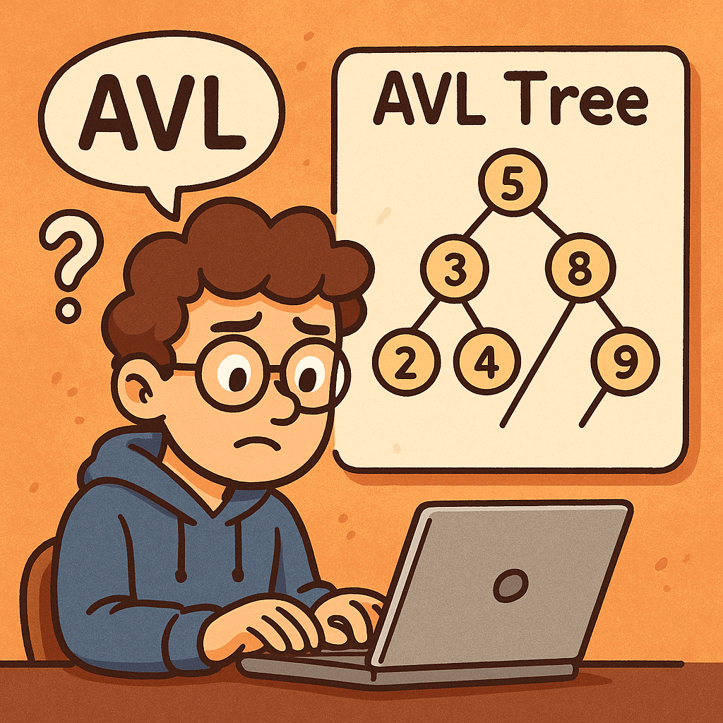
What is an AVL Tree?

An AVL tree (named after Adelson-Velsky and Landis) is a self-balancing Binary Search Tree (BST).
For every node, the balance factor (height of left subtree − height of right subtree) is constrained to −1, 0, or +1. When inserts or deletes break this rule, the tree rotates (LL, RR, LR, RL cases) to restore balance—keeping the height O(log n).

Key idea: By preventing the tree from becoming skewed, every search, insert, and delete stays fast and predictable.

When Do We Need It?

Use an AVL tree when you need ordered data with consistently fast lookups and you can afford a bit of extra work during updates:

  • Read-heavy workloads where searches dominate (e.g., 90% reads / 10% writes)
  • Realtime ranking/leaderboards where items must stay sorted
  • In-memory indexes (e.g., IDs, timestamps) for low-latency search and range queries
  • Autocomplete / prefix sets (when implemented over keys that must remain sorted)

Real-World Example

Imagine a price alert service maintaining thousands of stock tickers in memory, keyed by last-trade time.

  • Every incoming request asks, “What changed most recently?” or “Find the first ticker after time T.”
  • With an AVL tree, search and successor/predecessor queries remain O(log n) even during volatile trading, while rotations keep the structure balanced despite frequent inserts/deletes.

Main Operations and Complexity

Operations

  • Search(k) – standard BST search
  • Insert(k, v) – BST insert, then rebalance with rotations (LL, RR, LR, RL)
  • Delete(k) – BST delete (may replace with predecessor/successor), then rebalance
  • Find min/max, predecessor/successor, range queries

Time Complexity

  • Search: O(log n)
  • Insert: O(log n) (includes at most a couple of rotations)
  • Delete: O(log n) (may trigger rotations)
  • Min/Max, predecessor/successor: O(log n)

Space Complexity

  • Space: O(n) for nodes
  • Per-node overhead: O(1) (store height or balance factor)

Advantages

  • Guaranteed O(log n) for lookup, insert, delete (tighter balance than many alternatives)
  • Predictable latency under worst-case patterns (no pathologically skewed trees)
  • Great for read-heavy or latency-sensitive workloads

Disadvantages

  • More rotations/updates than looser trees (e.g., Red-Black) → slightly slower writes
  • Implementation complexity (more cases to handle correctly)
  • Cache locality worse than B-trees on disk; not ideal for large on-disk indexes

Quick Note on Rotations

  • LL / RR: one single rotation fixes it
  • LR / RL: a double rotation (child then parent) fixes it
    Rotations are local (affect only a few nodes) and keep the BST order intact.

AVL vs. (Plain) Binary Tree — What’s the Difference?

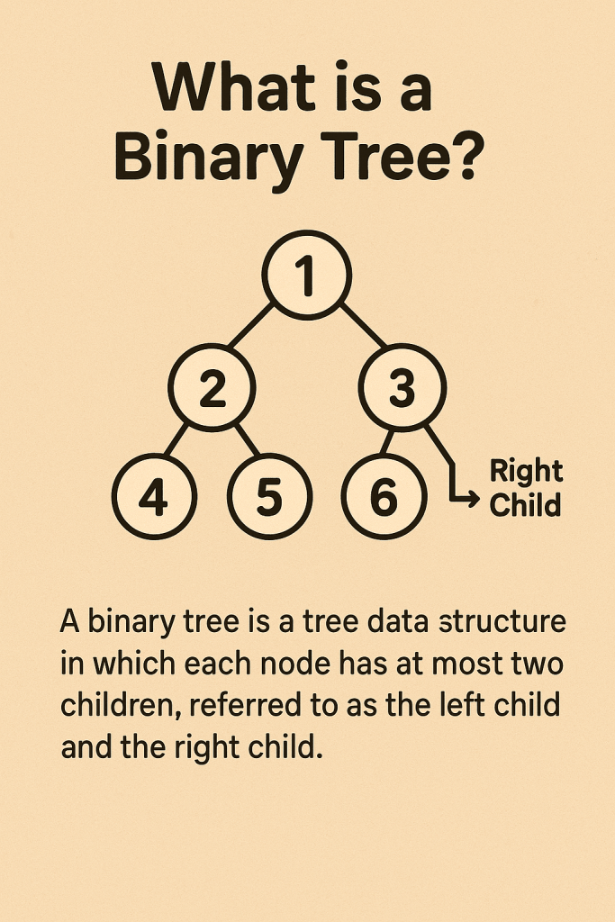
Many say “binary tree” when they mean “binary search tree (BST).” A plain binary tree has no ordering or balancing guarantees.
An AVL is a BST + balance rule that keeps height logarithmic.

FeaturePlain Binary TreeUnbalanced BSTAVL (Self-Balancing BST)
Ordering of keysNot requiredIn-order (left < node < right)In-order (left < node < right)
Balancing ruleNoneNoneHeight difference per node ∈ {−1,0,+1}
Worst-case heightO(n)O(n) (e.g., sorted inserts)O(log n)
SearchO(n) worst-caseO(n) worst-caseO(log n)
Insert/DeleteO(1)–O(n)O(1)–O(n)O(log n) (with rotations)
Update overheadMinimalMinimalModerate (rotations & height updates)
Best forSimple trees/traversalsWhen input is random and smallRead-heavy, latency-sensitive, ordered data

When to Prefer AVL Over Other Trees

  • Choose AVL when you must keep lookups consistently fast and don’t mind extra work on writes.
  • Choose Red-Black Tree when write throughput is a bit more important than the absolute tightness of balance.
  • Choose B-tree/B+-tree for disk-backed or paged storage.

Minimal Insert (Pseudo-Java) for Intuition

class Node {
  int key, height;
  Node left, right;
}

int h(Node n){ return n==null?0:n.height; }
int bf(Node n){ return n==null?0:h(n.left)-h(n.right); }
void upd(Node n){ n.height = 1 + Math.max(h(n.left), h(n.right)); }

Node rotateRight(Node y){
  Node x = y.left, T2 = x.right;
  x.right = y; y.left = T2;
  upd(y); upd(x);
  return x;
}
Node rotateLeft(Node x){
  Node y = x.right, T2 = y.left;
  y.left = x; x.right = T2;
  upd(x); upd(y);
  return y;
}

Node insert(Node node, int key){
  if(node==null) return new Node(){ {this.key=key; this.height=1;} };
  if(key < node.key) node.left = insert(node.left, key);
  else if(key > node.key) node.right = insert(node.right, key);
  else return node; // no duplicates

  upd(node);
  int balance = bf(node);

  // LL
  if(balance > 1 && key < node.left.key) return rotateRight(node);
  // RR
  if(balance < -1 && key > node.right.key) return rotateLeft(node);
  // LR
  if(balance > 1 && key > node.left.key){ node.left = rotateLeft(node.left); return rotateRight(node); }
  // RL
  if(balance < -1 && key < node.right.key){ node.right = rotateRight(node.right); return rotateLeft(node); }

  return node;
}

Summary

  • AVL = BST + strict balanceheight O(log n)
  • Predictable performance for search/insert/delete: O(log n)
  • Best for read-heavy or latency-critical ordered data; costs a bit more on updates.
  • Compared to a plain binary tree or unbalanced BST, AVL avoids worst-case slowdowns by design.

Binary Trees: A Practical Guide for Developers

A binary tree is a hierarchical data structure where each node has at most two children. It’s great for ordered data, fast lookups/insertions (often near O(log n)), and in-order traversal. With balancing (AVL/Red-Black), performance becomes reliably logarithmic. Downsides include pointer overhead and potential O(n) worst-cases if unbalanced.

What Is a Binary Tree?

A binary tree is a collection of nodes where:

  • Each node stores a value.
  • Each node has up to two child references: left and right.
  • The top node is the root; leaf nodes have no children.

Common variants

  • Binary Search Tree (BST): Left subtree values < node < right subtree values (enables ordered operations).
  • Balanced BSTs: (e.g., AVL, Red-Black) keep height ≈ O(log n) for consistent performance.
  • Heap (Binary Heap): Complete tree with heap property (parent ≤/≥ children); optimized for min/max retrieval, not for sorted in-order traversals.
  • Full/Complete/Perfect Trees: Structural constraints that affect height and storage patterns.

Key terms

  • Height (h): Longest path from root to a leaf.
  • Depth: Distance from root to a node.
  • Subtree: A tree formed by a node and its descendants.

When Do We Need It?

Use a binary tree when you need:

  • Ordered data with frequent inserts/lookups (BSTs).
  • Sorted iteration via in-order traversal without extra sorting.
  • Priority access (heaps for schedulers, caches, and task queues).
  • Range queries (e.g., “all keys between A and M”) more naturally than in hash maps.
  • Memory-efficient dynamic structure that grows/shrinks without contiguous arrays.

Avoid it when:

  • You only need exact-key lookups with no ordering → Hash tables may be simpler/faster on average.
  • Data is largely sequential/indexedArrays/ArrayLists can be better.

Real-World Example

Autocomplete suggestions (by prefix):

  1. Store words in a BST keyed by the word itself (or a custom key like (prefix, word)).
  2. To suggest completions for prefix “em”, find the lower_bound (“em…”) node, then do in-order traversal while keys start with “em”.
  3. This provides sorted suggestions with efficient insertions as vocabulary evolves.
    (If extreme scale/branching is needed, a trie may be even better—but BSTs are a simple, familiar starting point.)

Another quick one: Task scheduling with a min-heap (a binary heap). The smallest deadline pops first in O(log n), ideal for job schedulers.

Main Operations & Complexity

On a (possibly unbalanced) Binary Search Tree

OperationAverage TimeWorst TimeSpace (extra)
Search (find key)O(log n)O(n)O(1) iterative; O(h) recursive
InsertO(log n)O(n)O(1) / O(h)
DeleteO(log n)O(n)O(1) / O(h)
In-order/Preorder/Postorder TraversalO(n)O(n)O(h)
Level-order (BFS)O(n)O(n)O(w) (w = max width)
  • n = number of nodes, h = height of the tree (worst n−1), w = max nodes at any level.
  • A balanced BST keeps h ≈ log₂n, making search/insert/delete reliably O(log n).

On a Binary Heap

OperationTime
Push/InsertO(log n)
Pop Min/MaxO(log n)
Peek Min/MaxO(1)
Build-heap (from array)O(n)

Space for the tree overall is O(n). Traversals use O(h) stack space recursively (or O(1) if done iteratively with your own stack/queue memory accounted as O(n) in BFS).

Core Operations Explained (BST)

  • Search: Compare key at node; go left if smaller, right if larger; stop when equal or null.
  • Insert: Search where the key would be; attach a new node there.
  • Delete:
    • Leaf: remove directly.
    • One child: bypass node (link parent → child).
    • Two children: replace value with in-order successor (smallest in right subtree), then delete that successor node.
  • Traversal:
    • In-order (LNR): yields keys in sorted order.
    • Preorder (NLR): useful for serialization/cloning.
    • Postorder (LRN): useful for deletions/freeing.

Advantages

  • Near-logarithmic performance for search/insert/delete with balancing.
  • Maintains order → easy sorted iteration and range queries.
  • Flexible structure → no need for contiguous memory; easy to grow/shrink.
  • Rich ecosystem → balanced variants (AVL, Red-Black), heaps, treaps, etc.

Disadvantages

  • Unbalanced worst-case can degrade to O(n) (e.g., inserting sorted data into a naive BST).
  • Pointer overhead per node (vs. compact arrays).
  • More complex deletes than arrays/lists or hash maps.
  • Cache-unfriendly due to pointer chasing (vs. contiguous arrays/heaps).

Practical Tips

  • If you need reliably fast operations, choose a self-balancing BST (AVL or Red-Black).
  • For priority queues, use a binary heap (typically array-backed, cache-friendlier).
  • For prefix/string-heavy tasks, consider a trie; for exact lookups without ordering, consider a hash map.
  • Watch out for recursion depth with very deep trees; consider iterative traversals.

Summary

Binary trees sit at the heart of many performant data structures. Use them when ordering matters, when you want predictable performance (with balancing), and when sorted traversals or range queries are common. Pick the specific variant—BST, balanced BST, or heap—based on your dominant operations.

Blog at WordPress.com.

Up ↑