Search

Software Engineer's Notes

Author

eermisoglu

Understanding Model Context Protocol (MCP) and the Role of MCP Servers

What is Model Context Protocol?

The rapid evolution of AI tools—especially large language models (LLMs)—has brought a new challenge: how do we give AI controlled, secure, real-time access to tools, data, and applications?
This is exactly where the Model Context Protocol (MCP) comes into play.

In this blog post, we’ll explore what MCP is, what an MCP Server is, its history, how it works, why it matters, and how you can integrate it into your existing software development process.

MCP architecture

What Is Model Context Protocol?

Model Context Protocol (MCP) is an open standard designed to allow large language models to interact safely and meaningfully with external tools, data sources, and software systems.

Traditionally, LLMs worked with static prompts and limited context. MCP changes that by allowing models to:

  • Request information
  • Execute predefined operations
  • Access external data
  • Write files
  • Retrieve structured context
  • Extend their abilities through secure, modular “servers”

In short, MCP provides a unified interface between AI models and real software environments.

What Is a Model Context Protocol Server?

An MCP server is a standalone component that exposes capabilities, resources, and operations to an AI model through MCP.

Think of an MCP server as a plugin container, or a bridge between your application and the AI.

An MCP Server can provide:

  • File system access
  • Database queries
  • API calls
  • Internal business logic
  • Real-time system data
  • Custom actions (deploy, run tests, generate code, etc.)

MCP Servers work with any MCP-compatible LLM client (such as ChatGPT with MCP support), and they are configured with strict permissions for safety.

History of Model Context Protocol

Early Challenges with LLM Tooling

Before MCP, LLM tools were fragmented:

  • Every vendor used different APIs
  • Extensions were tightly coupled to the model platform
  • There was no standard for secure tool execution
  • Maintaining custom integrations was expensive

As developers started using LLMs for automation, code generation, and data workflows, the need for a secure, standardized protocol became clear.

Birth of MCP (2023–2024)

MCP originated from OpenAI’s efforts to unify:

  • Function calling
  • Extended tool access
  • Notebook-like interaction
  • File system operations
  • Secure context and sandboxing

The idea was to create a vendor-neutral protocol, similar to how REST standardized web communication.

Open Adoption and Community Growth (2024–2025)

By 2025, MCP gained widespread support:

  • OpenAI integrated MCP into ChatGPT clients
  • Developers started creating custom MCP servers
  • Tooling ecosystems expanded (e.g., filesystem servers, database servers, API servers)
  • Companies adopted MCP to give AI controlled internal access

MCP became a foundational building block for AI-driven software engineering workflows.

How Does MCP Work?

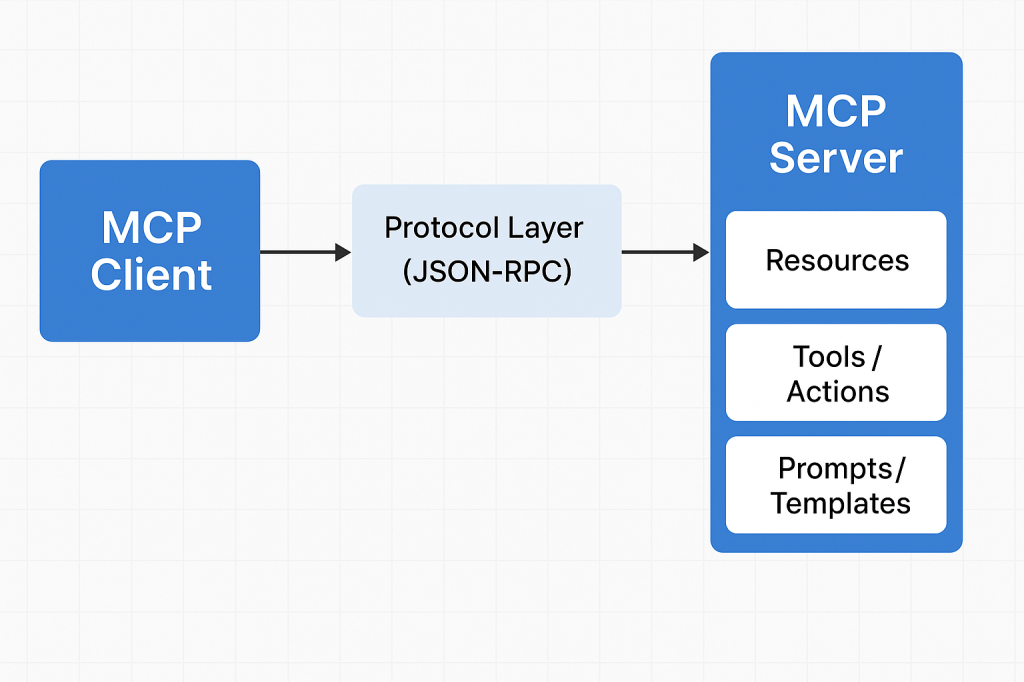
MCP works through a client–server architecture with clearly defined contracts.

1. The MCP Client

This is usually an AI model environment such as:

  • ChatGPT
  • VS Code AI extensions
  • IDE plugins
  • Custom LLM applications

The client knows how to communicate using MCP.

2. The MCP Server

Your MCP server exposes:

  • Resources → things the AI can reference
  • Tools / Actions → things the AI can do
  • Prompts / Templates → predefined workflows

Each server has permissions and runs in isolation for safety.

3. The Protocol Layer

Communication uses JSON-RPC over a standard channel (typically stdio or WebSocket).

The client asks:

“What tools do you expose?”

The server responds with:

“Here are resources, actions, and context you can use.”

Then the AI can call these tools securely.

4. Execution

When the AI executes an action (e.g., database query), the server performs the task on behalf of the model and returns structured results.

Why Do We Need MCP?

– Standardization

No more custom plugin APIs for each model. MCP is universal.

– Security

Strict capability control → AI only accesses what you explicitly expose.

– Extensibility

You can build your own MCP servers to extend AI.

– Real-time Interaction

Models can work with live:

  • data
  • files
  • APIs
  • business systems

– Sandbox Isolation

Servers run independently, protecting your core environment.

– Developer Efficiency

You can quickly create new AI-powered automations.

Benefits of Using MCP Servers

  • Reusable infrastructure — write once, use with any MCP-supported LLM.
  • Modularity — split responsibilities into multiple servers.
  • Portability — works across tools, IDEs, editor plugins, and AI platforms.
  • Lower maintenance — maintain one integration instead of many.
  • Improved automation — AI can interact with real systems (CI/CD, databases, cloud services).
  • Better developer workflows — AI gains accurate, contextual knowledge of your project.

How to Integrate MCP Into Your Software Development Process

1. Identify AI-Ready Tasks

Good examples:

  • Code refactoring
  • Automated documentation
  • Database querying
  • CI/CD deployment helpers
  • Environment setup scripts
  • File generation
  • API validation

2. Build a Custom MCP Server

Using frameworks like:

  • Node.js MCP Server Kits
  • Python MCP Server Kits
  • Custom implementations with JSON-RPC

Define what tools you want the model to access.

3. Expose Resources Safely

Examples:

  • Read-only project files
  • Specific database tables
  • Internal API endpoints
  • Configuration values

Always choose minimum required permissions.

4. Connect Your MCP Server to the Client

In ChatGPT or your LLM client:

  • Add local MCP servers
  • Add network MCP servers
  • Configure environment variables
  • Set up permissions

5. Use AI in Your Development Workflow

AI can now:

  • Generate code with correct system context
  • Run transformations
  • Trigger tasks
  • Help debug with real system data
  • Automate repetitive developer chores

6. Monitor and Validate

Use logging, audit trails, and usage controls to ensure safety.

Conclusion

Model Context Protocol (MCP) is becoming a cornerstone of modern AI-integrated software development. MCP Servers give LLMs controlled access to powerful tools, bridging the gap between natural language intelligence and real-world software systems.

By adopting MCP in your development process, you can unlock:

  • Higher productivity
  • Better automation
  • Safer AI integrations
  • Faster development cycles

Unit Testing: The What, Why, and How (with Practical Examples)

What is unit test?

What is a Unit Test?

A unit test verifies the smallest testable part of your software—usually a single function, method, or class—in isolation. Its goal is to prove that, for a given input, the unit produces the expected output and handles edge cases correctly.

Key characteristics

  • Small & fast: millisecond execution, in-memory.
  • Isolated: no real network, disk, or database calls.
  • Repeatable & deterministic: same input → same result.
  • Self-documenting: communicates intended behavior.

A Brief History (How We Got Here)

  • 1960s–1980s: Early testing practices emerged with procedural languages, but were largely ad-hoc and manual.
  • 1990s: Object-oriented programming popularized more modular designs. Kent Beck introduced SUnit for Smalltalk; the “xUnit” family was born.
  • Late 1990s–2000s: JUnit (Java) and NUnit (.NET) pushed unit testing mainstream. Test-Driven Development (TDD) formalized “Red → Green → Refactor.”
  • 2010s–today: Rich ecosystems (pytest, Jest, JUnit 5, RSpec, Go’s testing pkg). CI/CD and DevOps turned unit tests into a daily, automated safety net.

How Unit Tests Work (The Mechanics)

Arrange → Act → Assert (AAA)

  1. Arrange: set up inputs, collaborators (often fakes/mocks).
  2. Act: call the method under test.
  3. Assert: verify outputs, state changes, or interactions.

Test Doubles (isolate the unit)

  • Dummy: unused placeholders to satisfy signatures.
  • Stub: returns fixed data (no behavior verification).
  • Fake: lightweight implementation (e.g., in-memory repo).
  • Mock: verifies interactions (e.g., method X called once).
  • Spy: records calls for later assertions.

Good Test Qualities (FIRST)

  • Fast, Isolated, Repeatable, Self-Validating, Timely.

Naming & Structure

  • Name: methodName_condition_expectedResult
  • One assertion concept per test (clarity > cleverness).
  • Avoid coupling to implementation details (test behavior).

When Should We Write Unit Tests?

  • New code: ideally before or while coding (TDD).
  • Bug fixes: add a unit test that reproduces the bug first.
  • Refactors: guard existing behavior before changing code.
  • Critical modules: domain logic, calculations, validation.

What not to unit test

  • Auto-generated code, trivial getters/setters, framework wiring (unless it encodes business logic).

Advantages (Why Unit Test?)

  • Confidence & speed: safer refactors, fewer regressions.
  • Executable documentation: shows intended behavior.
  • Design feedback: forces smaller, decoupled units.
  • Lower cost of defects: catch issues early and cheaply.
  • Developer velocity: faster iteration with guardrails.

Practical Examples

Java (JUnit 5 + Mockito)

// src/test/java/com/example/PriceServiceTest.java
import org.junit.jupiter.api.Test;
import static org.junit.jupiter.api.Assertions.*;
import static org.mockito.Mockito.*;

class PriceServiceTest {
    @Test
    void applyDiscount_whenVIP_shouldReduceBy10Percent() {
        DiscountPolicy policy = mock(DiscountPolicy.class);
        when(policy.discountFor("VIP")).thenReturn(0.10);

        PriceService service = new PriceService(policy);
        double result = service.applyDiscount(200.0, "VIP");

        assertEquals(180.0, result, 0.0001);
        verify(policy, times(1)).discountFor("VIP");
    }
}

// Production code (for context)
class PriceService {
    private final DiscountPolicy policy;
    PriceService(DiscountPolicy policy) { this.policy = policy; }
    double applyDiscount(double price, String tier) {
        return price * (1 - policy.discountFor(tier));
    }
}
interface DiscountPolicy { double discountFor(String tier); }

Python (pytest)

# app/discount.py
def apply_discount(price: float, tier: str, policy) -> float:
    return price * (1 - policy.discount_for(tier))

# tests/test_discount.py
class FakePolicy:
    def discount_for(self, tier):
        return {"VIP": 0.10, "STD": 0.0}.get(tier, 0.0)

def test_apply_discount_vip():
    from app.discount import apply_discount
    result = apply_discount(200.0, "VIP", FakePolicy())
    assert result == 180.0

In-Memory Fakes Beat Slow Dependencies

// In-memory repository for fast unit tests
class InMemoryUserRepo implements UserRepo {
    private final Map<String, User> store = new HashMap<>();
    public void save(User u){ store.put(u.id(), u); }
    public Optional<User> find(String id){ return Optional.ofNullable(store.get(id)); }
}

Integrating Unit Tests into Your Current Process

1) Organize Your Project

/src
  /main
    /java (or /python, /ts, etc.)
  /test
    /java ...

  • Mirror package/module structure under /test.
  • Name tests after the unit: PriceServiceTest, test_discount.py, etc.

2) Make Tests First-Class in CI

GitHub Actions (Java example)

name: build-and-test
on: [push, pull_request]
jobs:
  test:
    runs-on: ubuntu-latest
    steps:
      - uses: actions/checkout@v4
      - uses: actions/setup-java@v4
        with: { distribution: temurin, java-version: '21' }
      - run: ./gradlew test --no-daemon

GitHub Actions (Python example)

name: pytest
on: [push, pull_request]
jobs:
  test:
    runs-on: ubuntu-latest
    steps:
      - uses: actions/checkout@v4
      - uses: actions/setup-python@v5
        with: { python-version: '3.12' }
      - run: pip install -r requirements.txt
      - run: pytest -q

3) Define “Done” with Tests

  • Pull requests must include unit tests for new/changed logic.
  • Code review checklist: readability, edge cases, negative paths.
  • Coverage gate (sensible threshold; don’t chase 100%).
    Example (Gradle + JaCoCo):
jacocoTestCoverageVerification {
    violationRules {
        rule { limit { counter = 'INSTRUCTION'; minimum = 0.75 } }
    }
}
test.finalizedBy jacocoTestReport, jacocoTestCoverageVerification

4) Keep Tests Fast and Reliable

  • Avoid real I/O; prefer fakes/mocks.
  • Keep each test < 100ms; whole suite in seconds.
  • Eliminate flakiness (random time, real threads, sleeps).

5) Use the Test Pyramid Wisely

  • Unit (broad base): thousands, fast, isolated.
  • Integration (middle): fewer, verify boundaries.
  • UI/E2E (tip): very few, critical user flows only.

A Simple TDD Loop You Can Adopt Tomorrow

  1. Red: write a failing unit test that expresses the requirement.
  2. Green: implement the minimum to pass.
  3. Refactor: clean design safely, keeping tests green.
  4. Repeat; keep commits small and frequent.

Common Pitfalls (and Fixes)

  • Mock-heavy tests that break on refactor → mock only at boundaries; prefer fakes for domain logic.
  • Testing private methods → test through public behavior; refactor if testing is too hard.
  • Slow suites → remove I/O, shrink fixtures, parallelize.
  • Over-asserting → one behavioral concern per test.

Rollout Plan (4 Weeks)

  • Week 1: Set up test frameworks, sample tests, CI pipeline, coverage reporting.
  • Week 2: Add tests for critical modules & recent bug fixes. Create a PR template requiring tests.
  • Week 3: Refactor hot spots guided by tests. Introduce an in-memory fake layer.
  • Week 4: Add coverage gates, stabilize the suite, document conventions in CONTRIBUTING.md.

Team Conventions

  • Folder structure mirrors production code.
  • Names: ClassNameTest or test_function_behavior.
  • AAA layout, one behavior per test.
  • No network/disk/DB in unit tests.
  • PRs must include tests for changed logic.

Final Thoughts

Unit tests pay dividends by accelerating safe change. Start small, keep them fast and focused, and wire them into your daily workflow (pre-commit, CI, PR reviews). Over time, they become living documentation and your best shield against regressions.

implements vs extends in Java

Difference between implements vs extends in Java

What does implements mean in Java?

An interface declares capabilities (method signatures, default methods, static methods, constants). A class uses implements to promise it provides those capabilities.

public interface Cache {
    Optional<String> get(String key);
    void put(String key, String value);
    default boolean contains(String key) { return get(key).isPresent(); }
}

public class InMemoryCache implements Cache {
    private final Map<String, String> store = new ConcurrentHashMap<>();
    public Optional<String> get(String key) { return Optional.ofNullable(store.get(key)); }
    public void put(String key, String value) { store.put(key, value); }
}

Key points:

  • A class can implement multiple interfaces: class A implements I1, I2 { ... }.
  • Interfaces can have default methods (since Java 8), helping evolve APIs without breaking implementors.
  • Records and enums can implement interfaces.
  • Interfaces cannot hold state (beyond public static final constants).

What does extends mean in Java?

1) Class → Class (single inheritance)

A class can extend one other class to reuse state/behavior and specialize it.

public abstract class Shape {
    public abstract double area();
}

public class Rectangle extends Shape {
    private final double w, h;
    public Rectangle(double w, double h) { this.w = w; this.h = h; }
    @Override public double area() { return w * h; }
}

2) Interface → Interface (multiple inheritance of type)

An interface can extend one or more interfaces to combine contracts.

public interface Startable { void start(); }
public interface Stoppable { void stop(); }
public interface Lifecycle extends Startable, Stoppable { }

Notes:

  • Classes cannot extend multiple classes.
  • Use super(...) to call a superclass constructor; use @Override to refine behavior.
  • If two parent interfaces provide the same default method, the implementing class must disambiguate by overriding.

Differences at a glance

Topicimplementsextends (class→class)extends (interface→interface)
PurposePromise behavior via interfaceReuse/ specialize implementation & stateCombine contracts
Multiple inheritanceClass can implement many interfacesNot allowed (single superclass)Allowed (an interface can extend many)
StateNo instance state in interfaceInherits fields and methodsNo instance state
ConstructorsN/ASubclass calls super(...)N/A
API evolutiondefault methods helpRisky; changes can rippledefault in parents propagate
Typical usePlug-in points, ports, test seamsTrue specialization (“is-a”)Build richer capability sets

When should I use each?

Use implements (interfaces) when:

  • You want flexible contracts decoupled from implementations (e.g., PaymentGateway, Cache, Repository).
  • You need multiple behaviors without tight coupling.
  • You care about testability (mock/fake implementations in unit tests).
  • You’re designing hexagonal/clean architecture ports and adapters.

Use extends (class inheritance) when:

  • There’s a strong “is-a” relationship and shared state/behavior that truly belongs in a base class.
  • You’re refining behavior of a framework base class (e.g., HttpServlet, Thread, java.io streams).
  • You need protected hooks / template methods for controlled extension.

Avoid overusing inheritance when composition (a field that delegates) is clearer and safer.

Why do we need them? Importance & benefits

  • Abstraction & decoupling: Interfaces let you program to capabilities, not concrete types, enabling swap-in implementations.
  • Reuse & specialization: Inheritance centralizes common behavior, reducing duplication (when it’s a true fit).
  • Polymorphism: Callers depend on supertype/interface; implementations can vary behind the scenes.
  • API evolution: Interfaces with default methods allow additive changes with fewer breaking changes.
  • Testability: Interfaces create clean boundaries for mocks/stubs; inheritance can provide test doubles via small overrides.

Practical examples (real-world flavored)

Spring Boot service port with an adapter

public interface EmailSender {
    void send(String to, String subject, String body);
}

@Service
public class SmtpEmailSender implements EmailSender {
    // inject JavaMailSender, etc.
    public void send(String to, String subject, String body) { /* ... */ }
}

// Usage: depend on EmailSender in controllers/use-cases, not on SMTP details.

Specializing a framework class (carefully)

public class AuditInputStream extends FilterInputStream {
    public AuditInputStream(InputStream in) { super(in); }
    @Override public int read() throws IOException {
        int b = super.read();
        // audit logic...
        return b;
    }
}

Modern features & gotchas

  • Default methods conflict: If A and B define the same default m(), a class implements A, B must override m() to resolve the diamond.
  • Abstract classes vs interfaces:
    • Use abstract classes when you need shared state, partial implementations, or constructors.
    • Use interfaces to define capabilities and support multiple inheritance of type.
  • Sealed classes (Java 17+): Control which classes can extend a base:
    public sealed class Token permits JwtToken, ApiKeyToken { }
  • Records: Can implements interfaces, great for DTOs with behavior contracts:
    public record Money(BigDecimal amount, Currency currency) implements Comparable<Money> { ... }

Integration into your team’s software development process

1) Architecture & layering

  • Define ports as interfaces in application/core modules (e.g., PaymentProcessor, UserRepository).
  • Implement adapters in infrastructure modules (JdbcUserRepository, StripePaymentProcessor).
  • Expose services via interfaces; keep controllers/use-cases depending on interfaces only.

2) Coding standards

  • Guideline: Prefer implements + composition; justify any extends in code review.
  • Naming: Interfaces describe capability (*Service, *Repository, *Gateway); implementations are specific (Jdbc*, S3*, InMemory*).
  • Visibility: Keep base classes package-private when possible; avoid protected fields.
  • Final classes/methods: Mark classes final unless a deliberate extension point.

3) Testing

  • Unit tests mock interfaces (Mockito/Stub implementations).
  • For inheritance, favor template methods and override only documented hooks in tests.

4) Code review checklist

  • Is this a true “is-a”? If not, prefer composition.
  • Are we depending on interfaces at boundaries?
  • Could an interface with a default help evolve this API safely?
  • Are we avoiding deep inheritance chains (max depth 1–2)?

5) Tooling & enforcement

  • Add static analysis rules (e.g., Error Prone/Checkstyle/Sonar) to flag deep inheritance and unused protected members.
  • Architectural tests (ArchUnit) to enforce “controllers depend on ports, not on adapters.”

Common pitfalls & how to avoid them

  • “God” base classes: Too much logic in a superclass → fragile subclasses. Split responsibilities; use composition.
  • Leaky abstractions: Interfaces that expose implementation details limit flexibility. Keep them capability-focused.
  • Over-mocking concrete classes: Depend on interfaces at boundaries to keep tests simple and fast.
  • Default method ambiguity: If combining interfaces with overlapping defaults, override explicitly.

FAQ

Can an interface extend a class?
No. Interfaces can only extend interfaces.

Can a class both extend and implement?
Yes: class C extends Base implements I1, I2 { ... }.

Is multiple inheritance supported?
For classes: no. For interfaces: yes (an interface may extend multiple interfaces; a class may implement multiple interfaces).

Interface vs abstract class—quick rule of thumb?
Need shared state/constructors → abstract class. Need flexible capability and multiple inheritance of type → interface.

Summary

  • Reach for implements to define what something can do.
  • Use extends to refine how something does it—only when it’s truly the same kind of thing.
  • Bake these choices into your architecture, guidelines, tests, and tooling to keep designs flexible and maintainable.

What Is CAPTCHA? Understanding the Gatekeeper of the Web

What Is CAPTCHA? Understanding the Gatekeeper of the Web

CAPTCHA — an acronym for Completely Automated Public Turing test to tell Computers and Humans Apart — is one of the most widely used security mechanisms on the internet. It acts as a digital gatekeeper, ensuring that users interacting with a website are real humans and not automated bots. From login forms to comment sections and online registrations, CAPTCHA helps maintain the integrity of digital interactions.

The History of CAPTCHA

The concept of CAPTCHA was first introduced in the early 2000s by a team of researchers at Carnegie Mellon University, including Luis von Ahn, Manuel Blum, Nicholas Hopper, and John Langford.

Their goal was to create a test that computers couldn’t solve easily but humans could — a reverse Turing test. The original CAPTCHAs involved distorted text images that required human interpretation.

Over time, as optical character recognition (OCR) technology improved, CAPTCHAs had to evolve to stay effective. This led to the creation of new types, including:

  • Image-based CAPTCHAs: Users select images matching a prompt (e.g., “Select all images with traffic lights”).
  • Audio CAPTCHAs: Useful for visually impaired users, playing distorted audio that needs transcription.
  • reCAPTCHA (2007): Acquired by Google in 2009, this variant helped digitize books and later evolved into reCAPTCHA v2 (“I’m not a robot” checkbox) and v3, which uses risk analysis based on user behavior.

Today, CAPTCHAs have become an essential part of web security and user verification worldwide.

How Does CAPTCHA Work?

At its core, CAPTCHA works by presenting a task that is easy for humans but difficult for bots. The system leverages differences in human cognitive perception versus machine algorithms.

The Basic Flow:

  1. Challenge Generation:
    The server generates a random challenge (e.g., distorted text, pattern, image selection).
  2. User Interaction:
    The user attempts to solve it (e.g., typing the shown text, identifying images).
  3. Verification:
    The response is validated against the correct answer stored on the server or verified using a third-party CAPTCHA API.
  4. Access Granted/Denied:
    If correct, the user continues the process; otherwise, the system requests another attempt.

Modern CAPTCHAs like reCAPTCHA v3 use behavioral analysis — tracking user movements, mouse patterns, and browsing behavior — to determine whether the entity is human without explicit interaction.

Why Do We Need CAPTCHA?

CAPTCHAs serve as a first line of defense against malicious automation and spam. Common scenarios include:

  • Preventing spam comments on blogs or forums.
  • Protecting registration and login forms from brute-force attacks.
  • Securing online polls and surveys from manipulation.
  • Protecting e-commerce checkouts from fraudulent bots.
  • Ensuring fair access to services like ticket booking or limited-edition product launches.

Without CAPTCHA, automated scripts could easily overload or exploit web systems, leading to security breaches, data misuse, and infrastructure abuse.

Challenges and Limitations of CAPTCHA

While effective, CAPTCHAs also introduce several challenges:

  • Accessibility Issues:
    Visually impaired users or users with cognitive disabilities may struggle with complex CAPTCHAs.
  • User Frustration:
    Repeated or hard-to-read CAPTCHAs can hurt user experience and increase bounce rates.
  • AI Improvements:
    Modern AI models, especially those using machine vision, can now solve traditional CAPTCHAs with >95% accuracy, forcing constant innovation.
  • Privacy Concerns:
    Some versions (like reCAPTCHA) rely on user behavior tracking, raising privacy debates.

Developers must balance security, accessibility, and usability when implementing CAPTCHA systems.

Real-World Examples

Here are some examples of CAPTCHA usage in real applications:

  • Google reCAPTCHA – Used across millions of websites to protect forms and authentication flows.
  • Cloudflare Turnstile – A privacy-focused alternative that verifies users without tracking.
  • hCaptcha – Offers website owners a reward model while verifying human interactions.
  • Ticketmaster – Uses CAPTCHA during high-demand sales to prevent bots from hoarding tickets.
  • Facebook and Twitter – Employ CAPTCHAs to block spam accounts and fake registrations.

Integrating CAPTCHA into Modern Software Development

Integrating CAPTCHA into your development workflow can be straightforward, especially with third-party APIs and libraries.

Step-by-Step Integration Example (Google reCAPTCHA v2):

  1. Register your site at Google reCAPTCHA Admin Console.
  2. Get the site key and secret key.
  3. Add the CAPTCHA widget in your frontend form:
<pre class="wp-block-syntaxhighlighter-code"><form action="verify.php" method="post">
  <div class="g-recaptcha" data-sitekey="YOUR_SITE_KEY"></div>
  <input type="submit" value="Submit">
</form>
<a href="https://www.google.com/recaptcha/api.js">https://www.google.com/recaptcha/api.js</a>
</pre>
  1. Verify the response in your backend (e.g., PHP, Python, Java):
import requests

response = requests.post(
    "https://www.google.com/recaptcha/api/siteverify",
    data={"secret": "YOUR_SECRET_KEY", "response": user_response}
)
result = response.json()
if result["success"]:
    print("Human verified!")
else:
    print("Bot detected!")

  1. Handle verification results appropriately in your application logic.

Integration Tips:

  • Combine CAPTCHA with rate limiting and IP reputation analysis for stronger security.
  • For accessibility, always provide audio or alternate options.
  • Use asynchronous validation to improve UX.
  • Avoid placing CAPTCHA on every form unnecessarily — use it strategically.

Conclusion

CAPTCHA remains a cornerstone of online security — balancing usability and protection. As automation and AI evolve, so must CAPTCHA systems. The shift from simple text challenges to behavior-based and privacy-preserving verification illustrates this evolution.

For developers, integrating CAPTCHA thoughtfully into the software development process can significantly reduce automated abuse while maintaining a smooth user experience.

MemorySanitizer (MSan): A Practical Guide for Finding Uninitialized Memory Reads

What is MemorySanitizer ?

What is MemorySanitizer?

MemorySanitizer (MSan) is a runtime instrumentation tool that flags reads of uninitialized memory in C/C++ (and languages that compile down to native code via Clang/LLVM). Unlike AddressSanitizer (ASan), which focuses on heap/stack/global buffer overflows and use-after-free, MSan’s sole mission is to detect when your program uses a value that was never initialized (e.g., a stack variable you forgot to set, padding bytes in a struct, or memory returned by malloc that you used before writing to it).

Common bug patterns MSan catches:

  • Reading a stack variable before assignment.
  • Using struct/class fields that are conditionally initialized.
  • Consuming library outputs that contain undefined bytes.
  • Leaking uninitialized padding across ABI boundaries.
  • Copying uninitialized memory and later branching on it.

How does MemorySanitizer work?

At a high level:

  1. Compiler instrumentation
    When you compile with -fsanitize=memory, Clang inserts checks and metadata propagation into your binary. Every program byte that could hold a runtime value gets an associated “shadow” state describing whether that value is initialized (defined) or not (poisoned).
  2. Shadow memory & poisoning
    • Shadow memory is a parallel memory space that tracks definedness of each byte in your program’s memory.
    • When you allocate memory (stack/heap), MSan poisons it (marks as uninitialized).
    • When you assign to memory, MSan unpoisons the relevant bytes.
    • When you read memory, MSan checks the shadow. If any bit is poisoned, it reports an uninitialized read.
  3. Taint/propagation
    Uninitialized data is treated like a taint: if you compute z = x + y and either x or y is poisoned, then z becomes poisoned. If poisoned data controls a branch or system call parameter, MSan reports it.
  4. Intercepted library calls
    Many libc/libc++ functions are intercepted so MSan can maintain correct shadow semantics—for example, telling MSan that memset to a constant unpoisons bytes, or that read() fills a buffer with defined data (or not, depending on return value). Using un-instrumented libraries breaks these guarantees (see “Issues & Pitfalls”).
  5. Origin tracking (optional but recommended)
    With -fsanitize-memory-track-origins=2, MSan stores an origin stack trace for poisoned values. When a bug triggers, you’ll see both:
    • Where the uninitialized read happens, and
    • Where the data first became poisoned (e.g., the stack frame where a variable was allocated but never initialized).
      This dramatically reduces time-to-fix.

Key Components (in detail)

  1. Compiler flags
    • Core: -fsanitize=memory
    • Origins: -fsanitize-memory-track-origins=2 (levels: 0/1/2; higher = richer origin info, more overhead)
    • Typical extras: -fno-omit-frame-pointer -g -O1 (or your preferred -O level; keep debuginfo for good stacks)
  2. Runtime library & interceptors
    MSan ships a runtime that:
    • Manages shadow/origin memory.
    • Intercepts popular libc/libc++ functions, syscalls, threading primitives, etc., to keep shadow state accurate.
  3. Shadow & Origin Memory
    • Shadow: tracks definedness per byte.
    • Origin: associates poisoned bytes with a traceable “birthplace” (function/file/line), invaluable for root cause.
  4. Reports & Stack Traces
    When MSan detects an uninitialized read, it prints:
    • The site of the read (file:line stack).
    • The origin (if enabled).
    • Register/memory dump highlighting poisoned bytes.
  5. Suppressions & Options
    • You can use suppressions for known noisy functions or third-party libs you cannot rebuild.
    • Runtime tuning via env vars (e.g., MSAN_OPTIONS) to adjust reporting, intercept behaviors, etc.

Issues, Limitations, and Gotchas

  • You must rebuild (almost) everything with MSan.
    If any library is not compiled with -fsanitize=memory (and proper flags), its interactions may produce false positives or miss bugs. This is the #1 hurdle.
    • In practice, you rebuild your app, its internal libraries, and as many third-party libs as feasible.
    • For system libs where rebuild is impractical, rely on interceptors and suppressions, but expect gaps.
  • Platform support is narrower than ASan.
    MSan primarily targets Linux and specific architectures. It’s less ubiquitous than ASan or UBSan. (Check your Clang/LLVM version’s docs for exact support.)
  • Runtime overhead.
    Expect ~2–3× CPU overhead and increased memory consumption, more with origin tracking. MSan is intended for CI/test builds—not production.
  • Focus scope: uninitialized reads only.
    MSan won’t detect buffer overflows, UAF, data races, UB patterns, etc. Combine with ASan/TSan/UBSan in separate jobs.
  • Struct padding & ABI wrinkles.
    Padding bytes frequently remain uninitialized and can “escape” via I/O, hashing, or serialization. MSan will flag these—sometimes noisy, but often uncovering real defects (e.g., nondeterministic hashes).

How and When Should We Use MSan?

Use MSan when:

  • You have flaky tests or heisenbugs suggestive of uninitialized data.
  • You want strong guarantees that values used in logic/branches/syscalls were actually initialized.
  • You’re developing security-sensitive or determinism-critical code (crypto, serialization, compilers, DB engines).
  • You’re modernizing a legacy codebase known to rely on “it happens to work”.

Workflow advice:

  • Run MSan in dedicated CI jobs on debug or rel-with-debinfo builds.
  • Combine with high-coverage tests, fuzzers, and scenario suites.
  • Keep origin tracking enabled in at least one job.
  • Incrementally port third-party deps or apply suppressions as you go.

FAQ

Q: Can I run MSan in production?
A: Not recommended. The overhead is significant and the goal is pre-production bug finding.

Q: What if I can’t rebuild a system library?
A: Try a source build, fall back to MSan interceptors and suppressions, or write wrappers that fully initialize buffers before/after calls.

Q: How does MSan compare to Valgrind/Memcheck?
A: MSan is compiler-based and much faster, but requires recompilation. Memcheck is binary-level (no recompile) but slower; using both in different pipelines is often valuable.

Conclusion

MemorySanitizer is laser-focused on a class of bugs that can be subtle, security-relevant, and notoriously hard to reproduce. With a dedicated CI job, origin tracking, and disciplined rebuilds of dependencies, MSan will pay for itself quickly—turning “it sometimes fails” into a concrete stack trace and a one-line fix.

Sample Ratio Mismatch (SRM) in A/B Testing

What is Sample Ratio Mismatch?

What is Sample Ratio Mismatch?

Sample Ratio Mismatch (SRM) is when the observed allocation of users to variants differs significantly from the planned allocation.
Example: You configured a 50/50 split, but after 10,000 users you see 5,300 in A and 4,700 in B. That’s likely SRM.

SRM means the randomization or eligibility pipeline is biased (or data capture is broken), so any effect estimates (lift, p-values, etc.) can’t be trusted.

How SRM Works (Conceptually)

When you specify a target split like 50/50 or 33/33/34, each incoming unit (user, device, session, etc.) should be randomly bucketed so that the expected distribution matches your target in expectation.

Formally, for a test with k variants and total N assigned units, the expected count for variant i is:

E_i = p_i N

where

p_i is the target proportion for variant 𝑖 i and N

is the total sample size.

If the observed counts,

O_i

, differ from the expected more than chance alone would allow, you have an SRM.

How to Identify SRM (Step-by-Step)

1) Use a Chi-Square Goodness-of-Fit Test (recommended)

For k variants, compute:

χ2 = ( (O_iE_i)2 E_i )

with degrees of freedom df=k−1. Compute the p-value from the chi-square distribution. If the p-value is very small (common thresholds: 10−3 to 10−6), you’ve likely got an SRM.

Example (two-arm 50/50):
N=10,000,  OA=5,300,  OB=4,700,  EA=EB=5,000

χ2 = (5300-5000)^2 5000 + (4700-5000)^2 5000 =36

With df=1, p≈1.97×10⁻⁹. This triggers SRM.

2) Visual/Operational Checks

  • Live split dashboard: Show observed vs. expected % by variant.
  • Stratified checks: Repeat the chi-square by country, device, browser, app version, traffic source, time-of-day to find where the skew originates.
  • Time series: Plot cumulative allocation over time—SRM that “drifts” may indicate a rollout, caching, or traffic-mix issue.

3) Early-Warning Rule of Thumb

If your observed proportion deviates from the target by more than a few standard errors early in the test, investigate. For two arms with target p=0.5, the sampling variance under perfect randomization is:

σp = p(1p) N

Large persistent deviations → likely SRM.

Common Causes of SRM

  1. Eligibility asymmetry: Filters (geo, device, login state, new vs. returning) applied after assignment or applied differently per variant.
  2. Randomization at the wrong unit: Assigning by session but analyzing by user (or vice versa); cross-device users collide.
  3. Inconsistent hashing/salts: Different hash salt/seed per service or per page; some code paths skip/override the assignment.
  4. Sticky sessions / caching / CDNs: Edge caching or load balancer stickiness pinning certain users to one variant.
  5. Traffic shaping / rollouts: Feature flags, canary releases, or time-based rollouts inadvertently biasing traffic into one arm.
  6. Bot or test traffic: Non-human or QA traffic not evenly distributed (or filtered in one arm only).
  7. Telemetry loss / logging gaps: Events dropped more in one arm (ad-blockers, blocked endpoints, CORS, mobile SDK bugs).
  8. User-ID vs. device-ID mismatch: Some users bucketed by cookie, others by account ID; cookie churn changes ratios.
  9. Late triggers: Assignment happens at “conversion event” time in one arm but at page load in another.
  10. Geo or platform routing differences: App vs. web, iOS vs. Android, or specific regions routed to different infrastructure.

How to Prevent SRM (Design & Implementation)

  • Choose the right unit of randomization (usually user). Keep it consistent from assignment through analysis.
  • Server-side assignment with deterministic hashing on a stable ID (e.g., user_id). Example mapping:
b= { A if (H(user\_id||salt)modM)<pM B otherwise }

where H is a stable hash, M a large modulus (e.g., 106), and p the target proportion for A.

  • Single source of truth for assignment (SDKs/services call the same bucketing service).
  • Pre-exposure assignment: Decide the variant before any UI/network differences occur.
  • Symmetric eligibility: Apply identical inclusion/exclusion filters before assignment.
  • Consistent rollout & flags: If you use gradual rollouts, do it outside the experiment or symmetrically across arms.
  • Bot/QA filtering: Detect and exclude bots and internal IPs equally for all arms.
  • Observability: Log (unit_id, assigned_arm, timestamp, eligibility_flags, platform, geo) to a central stream. Monitor split, by segment, in real time.
  • Fail-fast alerts: Trigger alerts when SRM p-value falls below a strict threshold (e.g., p<10−4).

How to Fix SRM (Triage & Remediation)

  1. Pause the experiment immediately. Do not interpret effect estimates from an SRM-affected test.
  2. Localize the bias. Recompute chi-square by segment (geo, device, source). The segment with the strongest SRM often points to the root cause.
  3. Audit the assignment path.
    • Verify the unit ID is consistent (user_id vs. cookie).
    • Check hash function + salt are identical everywhere.
    • Ensure assignment occurs pre-render and isn’t skipped due to timeouts.
  4. Check eligibility filters. Confirm identical filters are applied before assignment and in both arms.
  5. Review infra & delivery. Look for sticky sessions, CDN cache keys, or feature flag rollouts that differ by arm.
  6. Inspect telemetry. Compare event loss rates by arm/platform. Fix SDK/network issues (e.g., batch size, retry logic, CORS).
  7. Sanitize traffic. Exclude bots/internal traffic uniformly; re-run SRM checks.
  8. Rerun a smoke test. After fixes, run a small, short dry-run experiment to confirm the split is healthy (no SRM) before relaunching the real test.

Analyst’s Toolkit (Ready-to-Use)

  • SRM Chi-Square (two-arm 50/50):
χ2 = (O_AN/2)2 N/2 + (O_BN/2)2 N/2
  • General kkk-arm expected counts:
E_i=p_iN
  • Standard error for a two-arm proportion (target ppp):
σp= p(1p) N

Practical Checklist

  • Confirm unit of randomization and use stable IDs.
  • Perform server-side deterministic hashing with shared salt.
  • Apply eligibility before assignment, symmetrically.
  • Exclude bots/QA consistently.
  • Instrument SRM alerts (e.g., chi-square p<10−4).
  • Segment SRM monitoring by platform/geo/source/time.
  • Pause & investigate immediately if SRM triggers.

Summary

SRM isn’t a minor annoyance—it’s a stop sign. It tells you that the randomization or measurement is broken, which can fabricate uplifts or hide regressions. Detect it early with a chi-square test, design your experiments to prevent it (stable IDs, deterministic hashing, symmetric eligibility), and never ship decisions from an SRM-affected test.

Unit of Randomization in A/B Testing: A Practical Guide

What is unit of randomization?

What is a “Unit of Randomization”?

The unit of randomization is the entity you randomly assign to variants (A or B). It’s the “thing” that receives the treatment: a user, a session, a device, a household, a store, a geographic region, etc.

Choosing this unit determines:

  • Who gets which experience
  • How independence assumptions hold (or break)
  • How you compute statistics and sample size
  • How actionable and unbiased your results are

How It Works (at a high level)

  1. Define exposure: decide what entity must see a consistent experience (e.g., “Logged-in user must always see the same variant across visits.”).
  2. Create an ID: select an identifier for that unit (e.g., user_id, device_id, household_id, store_id).
  3. Hash & assign: use a stable hashing function to map each ID into variant A or B with desired split (e.g., 50/50).
  4. Persist: ensure the unit sticks to its assigned variant on every exposure (stable bucketing).
  5. Analyze accordingly: aggregate metrics at or above the unit level; use the right variance model (especially for clusters).

Common Units of Randomization (with pros/cons and when to use)

1) User-Level (Account ID or Login ID)

  • What it is: Each unique user/account is assigned to a variant.
  • Use when: Logged-in products; experiences should persist across devices and sessions.
  • Pros: Clean independence between users; avoids cross-device contamination for logged-in flows.
  • Cons: Requires reliable, unique IDs; guest traffic may be excluded or need fallback logic.

2) Device-Level (Device ID / Mobile Advertiser ID)

  • What it is: Each physical device is assigned.
  • Use when: Native apps; no login, but device ID is stable.
  • Pros: Better than cookies for persistence; good for app experiments.
  • Cons: Same human on multiple devices may see different variants; may bias human-level metrics.

3) Cookie-Level (Browser Cookie)

  • What it is: Each browser cookie gets a variant.
  • Use when: Anonymous web traffic without login.
  • Pros: Simple to implement.
  • Cons: Cookies expire/clear; users have multiple browsers/devices → contamination and assignment churn.

4) Session-Level

  • What it is: Each session is randomized; the same user may see different variants across sessions.
  • Use when: You intentionally want short-lived treatment (e.g., page layout in a one-off landing funnel).
  • Pros: Fast ramp, lots of independent observations.
  • Cons: Violates persistence; learning/carryover effects make interpretation tricky for longer journeys.

5) Pageview/Request-Level

  • What it is: Every pageview or API request is randomized.
  • Use when: Low-stakes UI tweaks with negligible carryover; ads/creative rotation tests.
  • Pros: Maximum volume quickly.
  • Cons: Massive contamination; not suitable when the experience should be consistent within a visit.

6) Household-Level

  • What it is: All members/devices of a household share the same assignment (derived from address or shared account).
  • Use when: TV/streaming, grocery delivery, multi-user homes.
  • Pros: Limits within-home interference; aligns with purchase behavior.
  • Cons: Hard to define reliably; potential privacy constraints.

7) Network/Team/Organization-Level

  • What it is: Randomize at a group/organization level (e.g., company admin sets a feature; all employees see it).
  • Use when: B2B products; settings that affect the whole group.
  • Pros: Avoids spillovers inside an org.
  • Cons: Fewer units → lower statistical power; requires cluster-aware analysis.

8) Geographic/Store/Region-Level (Cluster Randomization)

  • What it is: Entire locations are assigned (cities, stores, countries, data centers).
  • Use when: Pricing, inventory, logistics, or features tied to physical/geo constraints.
  • Pros: Realistic operational measurement, cleaner separation across regions.
  • Cons: Correlated outcomes within a cluster; requires cluster-robust analysis and typically larger sample sizes.

Why the Unit of Randomization Matters

1) Validity (Independence & Interference)

Statistical tests assume independent observations. If people in the control are affected by those in treatment (interference), estimates are biased. Picking a unit that contains spillovers (e.g., randomize at org or store level) preserves validity.

2) Power & Sample Size (Design Effect)

Clustered units (households, stores, orgs) share similarities—captured by intra-class correlation (ICC), often denoted ρ\rhoρ. This inflates variance via the design effect:

DE = 1 + ( m 1 ) ρ

Where m is the average cluster size. Your effective sample size becomes:

neff = n DE

Larger clusters or higher ρ → bigger DE → less power for the same raw n.

3) Consistency of Experience

Units like user-level + stable bucketing ensure a user’s experience doesn’t flip between variants, avoiding dilution and confusion.

4) Interpretability & Actionability

If you sell at the store level, store-level randomization makes metrics easier to translate into operational decisions. If you optimize user engagement, user-level makes more sense.

How to Choose the Right Unit (Decision Checklist)

  • Where do spillovers happen?
    Pick the smallest unit that contains meaningful interference (user ↔ household ↔ org ↔ region).
  • What is the primary decision maker?
    If rollouts happen per account/org/region, align the unit with that boundary.
  • Can you persist assignment?
    Use stable identifiers and hashing (e.g., SHA-256 on user_id + experiment_name) to keep assignments sticky.
  • How will you analyze it?
    • User/cookie/device: standard two-sample tests aggregated per unit.
    • Cluster (org/store/geo): use cluster-robust standard errors or mixed-effects models; adjust for design effect in planning.
  • Is the ID reliable & unique?
    Prefer user_id over cookie when possible. If only cookies exist, add fallbacks and measure churn.

Practical Implementation Tips

  • Stable Bucketing: Hash the chosen unit ID to a uniform number in [0,1); map ranges to variants (e.g., <0.5 → A, ≥0.5 → B). Store assignment server-side for reliability.
  • Cross-Device Consistency: If the same human might use multiple devices, prefer user-level (requires login) or implement a linking strategy (e.g., email capture) before randomization.
  • Exposure Control: Ensure treatment is only applied after assignment; log exposures to avoid partial-treatment bias.
  • Metric Aggregation: Aggregate outcomes per randomized unit first (e.g., user-level conversion), then compare arms. Avoid pageview-level analysis when randomizing at user level.
  • Bot & Duplicate Filtering: Scrub bots and detect duplicate IDs (e.g., shared cookies) to reduce contamination.
  • Pre-Experiment Checks: Verify balance on key covariates (traffic source, device, geography) across variants for the chosen unit.

Examples

  • Pricing test in retail chain → randomize at store level; compute sales per store; analyze with cluster-robust errors; account for region seasonality.
  • New signup flow on a web app → randomize at user level (or cookie if anonymous); ensure users see the same variant across sessions.
  • Homepage hero image rotation for paid ads landing page → potentially session or pageview level; keep awareness of contamination if users return.

Common Pitfalls (and how to avoid them)

  • Using too granular a unit (pageview) for features with memory/carryover → inconsistent experiences and biased results.
    Fix: move to session or user level.
  • Ignoring clustering when randomizing stores/teams → inflated false positives.
    Fix: use cluster-aware analysis and plan for design effect.
  • Cookie churn breaks persistence → variant switching mid-experiment.
    Fix: server-side assignment with long-lived identifiers; encourage login.
  • Interference across units (social/network effects) → contamination.
    Fix: enlarge the unit (household/org/region) or use geo-experiments with guard zones.

Frequentist Inference in A/B Testing: A Practical Guide

What is Frequentist ?

What is “Frequentist” in A/B Testing?

Frequentist inference interprets probability as the long-run frequency of events. In the context of A/B tests, it asks: If I repeatedly ran this experiment under the null hypothesis, how often would I observe a result at least this extreme just by chance?
Key objects in the frequentist toolkit are null/alternative hypotheses, test statistics, p-values, confidence intervals, Type I/II errors, and power.

Core Concepts (Fast Definitions)

  • Null hypothesis (H₀): No difference between variants (e.g., pA=pB​).
  • Alternative hypothesis (H₁): There is a difference (two-sided) or a specified direction (one-sided).
  • Test statistic: A standardized measure (e.g., a z-score) used to compare observed effects to what chance would produce.
  • p-value: Probability, assuming H₀ is true, of observing data at least as extreme as what you saw.
  • Significance level (α): Threshold for rejecting H₀ (often 0.05).
  • Confidence interval (CI): A range of plausible values for the effect size that would capture the true effect in X% of repeated samples.
  • Power (1−β): Probability your test detects a true effect of a specified size (i.e., avoids a Type II error).

How Frequentist A/B Testing Works (Step-by-Step)

1) Define the effect and hypotheses

For a proportion metric like conversion rate (CR):

  • pA​ = baseline CR (variant A/control)
  • pB​ = treatment CR (variant B/experiment)

Null hypothesis:

H0:pA=pB

Two-sided alternative:

H1:pApB

2) Choose α, power, and (optionally) the Minimum Detectable Effect (MDE)

  • Common choices: α = 0.05, power = 0.8 or 0.9.
  • MDE is the smallest lift you care to detect (planning parameter for sample size).

3) Collect data according to a pre-registered plan

Let nA,nB​ be samples; xA,xB​ conversions; pA=xA/nA, pB=xB/nB.

4) Compute the test statistic (two-proportion z-test)

Pooled proportion under H₀:

p=xA+xBnA+nB

Standard error (SE) under H₀:

SE=p(1p)×(1nA+1nB)

z-statistic:

z=(pBpA)SE

5) Convert z to a p-value

For a two-sided test:

p−value=2×(1Φ(z))

where Φ is the standard normal CDF.

6) Decision rule

  • If p-value ≤ α ⇒ Reject H₀ (evidence of a difference).
  • If p-value > α ⇒ Fail to reject H₀ (data are consistent with no detectable difference).

7) Report the effect size with a confidence interval

Approximate 95% CI for the difference (pB−pA):

(pBpA)±1.96×pA(1pA)nA+pB(1pB)nB

Tip: Also report relative lift (pB/pA−1) and absolute difference (pB−pA).

A Concrete Example (Conversions)

Suppose:

  • nA=10,000,  xA=900⇒pA=0.09
  • nB=10,000,  xB=960⇒pB=0.096

Compute pooled p​, SE, z, p-value, CI using the formulas above. If the two-sided p-value ≤ 0.05 and the CI excludes 0, you can conclude a statistically significant lift of ~0.6 percentage points (≈6.7% relative).

Why Frequentist Testing Is Important

  1. Clear, widely-understood decisions
    Frequentist tests provide a familiar yes/no decision rule (reject/fail to reject H₀) that is easy to operationalize in product pipelines.
  2. Error control at scale
    By fixing α, you control the long-run rate of false positives (Type I errors), crucial when many teams run many tests.
TypeIerrorrate=α
  1. Confidence intervals communicate uncertainty
    CIs provide a range of plausible effects, helping stakeholders gauge practical significance (not just p-values).
  2. Power planning avoids underpowered tests
    You can plan sample sizes to hit desired power for your MDE, reducing wasted time and inconclusive results.

Approximate two-sample proportion power-based sample size per variant:

n(z1−α/2×2p(1p)+z power×p(1p)+(p+Δ)(1pΔ))Δ2

where p is baseline CR and Δ is your MDE in absolute terms.

Practical Guidance & Best Practices

  • Pre-register your hypothesis, metrics, α, stopping rule, and analysis plan.
  • Avoid peeking (optional stopping inflates false positives). If you need flexibility, use group-sequential or alpha-spending methods.
  • Adjust for multiple comparisons when testing many variants/metrics (e.g., Bonferroni, Holm, or control FDR).
  • Check metric distributional assumptions. For very small counts, prefer exact or mid-p tests; for large samples, z-tests are fine.
  • Report both statistical and practical significance. A tiny but “significant” lift may not be worth the engineering cost.
  • Monitor variance early. High variance metrics (e.g., revenue/user) may require non-parametric tests or transformations.

Frequentist vs. Bayesian

  • Frequentist p-values tell you how unusual your data are if H₀ were true.
  • Bayesian methods provide a posterior distribution for the effect (e.g., probability the lift > 0).
    Both are valid; frequentist tests remain popular for their simplicity, well-established error control, and broad tooling support.

Common Pitfalls & How to Avoid Them

  • Misinterpreting p-values: A p-value is not the probability H₀ is true.
  • Multiple peeks without correction: Inflates Type I errors—use planned looks or sequential methods.
  • Underpowered tests: Leads to inconclusive results—plan with MDE and power.
  • Metric shift & novelty effects: Run long enough to capture stabilized user behavior.
  • Winner’s curse: Significant early winners may regress—replicate or run holdout validation.

Reporting Template

  • Hypothesis: H0:pA=pB, H1​: two-sided
  • Design: α=0.05, power=0.8, MDE=…
  • Data: nA,xA,pA; nB,xB,pB
  • Analysis: two-proportion z-test (pooled), 95% CI
  • Result: p-value = …, z = …, 95% CI = […, …], effect = absolute … / relative …
  • Decision: reject/fail to reject H₀
  • Notes: peeking policy, multiple-test adjustments, assumptions check

Final Takeaway

Frequentist A/B testing gives you a disciplined framework to decide whether a product change truly moves your metric or if the observed lift could be random noise. With clear error control, simple decision rules, and mature tooling, it remains a workhorse for experimentation at scale.

Stable Bucketing in A/B Testing

What is Stable Bucketing?

What Is Stable Bucketing?

Stable bucketing is a repeatable, deterministic way to assign units (users, sessions, accounts, devices, etc.) to experiment variants so that the same unit always lands in the same bucket whenever the assignment is recomputed. It’s typically implemented with a hash function over a unit identifier and an experiment “seed” (or namespace), then mapped to a bucket index.

Key idea: assignment never changes for a given (unit_id, experiment_seed) unless you deliberately change the seed or unit of bucketing. This consistency is crucial for clean experiment analysis and operational simplicity.

Why We Need It (At a Glance)

  • Consistency: Users don’t flip between A and B when they return later.
  • Reproducibility: You can recompute assignments offline for debugging and analysis.
  • Scalability: Works statelessly across services and languages.
  • Safety: Lets you ramp traffic up or down without re-randomizing previously assigned users.
  • Analytics integrity: Reduces bias and cross-contamination when users see multiple experiments.

How Stable Bucketing Works (Step-by-Step)

1) Choose Your Unit of Bucketing

Pick the identity that best matches the causal surface of your treatment:

  • User ID (most common): stable across sessions/devices (if you have login).
  • Device ID: when login is rare; beware of cross-device spillover.
  • Session ID / Request ID: only for per-request or per-session treatments.

Rule of thumb: bucket at the level where the treatment is applied and outcomes are measured.

2) Build a Deterministic Hash

Compute a hash over a canonical string like:

canonical_key = experiment_namespace + ":" + unit_id
hash = H(canonical_key)  // e.g., 64-bit MurmurHash3, xxHash, SipHash

Desiderata: fast, language-portable implementations, low bias, and uniform output over a large integer space (e.g., 2^64).

3) Normalize to [0, 1)

Convert the integer hash to a unit interval. With a 64-bit unsigned hash h∈{0,…,264−1}:

u = h / 2^64   // floating-point in [0,1)

4) Map to Buckets

If you have K total buckets (e.g., 1000) and want to allocate N of them to the experiment (others remain “control” or “not in experiment”), you can map:

bucket = u × K

Then assign variant ranges. For a 50/50 split with two variants A and B over the same experiment allocation, for example:

  • A gets buckets [0,K/2−1]
  • B gets buckets [K/2,K−1]

You can also reserve a global “control” by giving it a fixed bucket range that is outside any experiment’s allocation.

5) Control Allocation (Traffic Percentage)

If the intended inclusion probability is p (e.g., 10%), assign the first p⋅K buckets to the experiment:

N = p × K

Include a unit if bucket < N. Split inside N across variants according to desired proportions.

Minimal Pseudocode (Language-Agnostic)

function assign_variant(unit_id, namespace, variants):
    // variants = [{name: "A", weight: 0.5}, {name: "B", weight: 0.5}]
    key = namespace + ":" + canonicalize(unit_id)
    h = Hash64(key)                       // e.g., MurmurHash3 64-bit
    u = h / 2^64                          // float in [0,1)
    // cumulative weights to pick variant
    cum = 0.0
    for v in variants:
        cum += v.weight
        if u < cum:
            return v.name
    return variants[-1].name              // fallback for rounding

Deterministic: same (unit_id, namespace) → same u → same variant every time.

Statistical Properties (Why It Works)

Assuming the hash behaves like a uniform random function over [0,1), the inclusion indicator li​ for each unit i with target probability p is:

(A) = E[n_A] = pn Var[n_A] = np(1p)

With stable bucketing, units included at ramp-up remain included as you increase p (monotone ramps), which avoids re-randomization noise.

Benefits & Why It’s Important (In Detail)

1) User Experience Consistency

  • A returning user continues to see the same treatment, preventing confusion and contamination.
  • Supports long-running or incremental rollouts (10% → 25% → 50% → 100%) without users flipping between variants.

2) Clean Causal Inference

  • Avoids cross-over effects that can bias estimates when users switch variants mid-experiment.
  • Ensures SUTVA-like stability at the chosen unit (no unit’s potential outcomes change due to assignment instability).

3) Operational Simplicity & Scale

  • Stateless assignment (derive on the fly from (unit_id, namespace)).
  • Works across microservices and languages as long as the hash function and namespace are shared.

4) Reproducibility & Debugging

  • Offline recomputation lets you verify assignments, investigate suspected sample ratio mismatches (SRM), and audit exposure logs.

5) Safe Traffic Management

  • Ramps: increasing p simply widens the bucket interval—no reshuffling of already exposed users.
  • Kill-switches: setting p=0 instantly halts new exposures while keeping analysis intact.

6) Multi-Experiment Harmony

  • Use namespaces or layered bucketing to keep unrelated experiments independent while permitting intended interactions when needed.

Practical Design Choices & Pitfalls

Hash Function

  • Prefer fast, well-tested non-cryptographic hashes (MurmurHash3, xxHash).
  • If adversarial manipulation is a risk (e.g., public IDs), consider SipHash or SHA-based hashing.

Namespace (Seed) Discipline

  • The experiment_namespace must be unique per experiment/phase. Changing it intentionally re-randomizes.
  • For follow-up experiments requiring independence, use a new namespace. For continued exposure, reuse the old one.

Bucket Count & Mapping

  • Use a large K (e.g., 10,000) to get fine-grained control over traffic percentages and reduce allocation rounding issues.

Unit of Bucketing Mismatch

  • If treatment acts at the user level but you bucket by device, a single user on two devices can see different variants (spillover). Align unit with treatment.

Identity Resolution

  • Cross-device/user-merges can change effective unit IDs. Decide whether to lock assignment post-merge or recompute at login—document the policy and its analytical implications.

SRM Monitoring

  • Even with stable bucketing, instrumentation bugs, filters, and eligibility rules can create SRM. Continuously monitor observed splits versus expected ppp.

Privacy & Compliance

  • Hash only pseudonymous identifiers and avoid embedding raw PII in logs. Salt/namespace prevents reuse of the same hash across experiments.

Example: Two-Variant 50/50 with 20% Traffic

Setup

  • K=10,000 buckets
  • Experiment gets p=0.2 ⇒ N=2,000 buckets
  • Within experiment, A and B each get 50% of the N buckets (1,000 each)

Mapping

  • Include user if 0 ≤ bucket < 2000
  • If included:
    • A: 0 ≤ bucket < 1000
    • B: 1000 ≤ bucket < 2000
  • Else: not in experiment (falls through to global control)

Ramp from 20% → 40%

  • Extend inclusion to 0 ≤ bucket < 4000
  • Previously included users stay included; new users are added without reshuffling earlier assignments.

Math Summary (Allocation & Variant Pick)

Inclusion Decision

include = [ u×K < N ]

Variant Selection by Cumulative Weights

Let variants have weights w1,…wm​ with ∑wj=1 . Pick the smallest j such that:

u < k=1 wk

Implementation Tips (Prod-Ready)

  • Canonicalization: Lowercase IDs, trim whitespace, and normalize encodings before hashing.
  • Language parity tests: Create cross-language golden tests (input → expected bucket) for your SDKs.
  • Versioning: Version your bucketing algorithm; log algo_version, namespace, and unit_id_type.
  • Exposure logs: Record (unit_id, namespace, variant, timestamp) for auditability.
  • Dry-run: Add an endpoint or feature flag to validate expected split on synthetic data before rollout.

Takeaways

Stable bucketing is the backbone of reliable A/B testing infrastructure. By hashing a stable unit ID within a disciplined namespace, you get deterministic, scalable, and analyzable assignments. This prevents cross-over effects, simplifies rollouts, and preserves statistical validity—exactly what you need for trustworthy product decisions.

Blog at WordPress.com.

Up ↑