Software Engineer's Notes

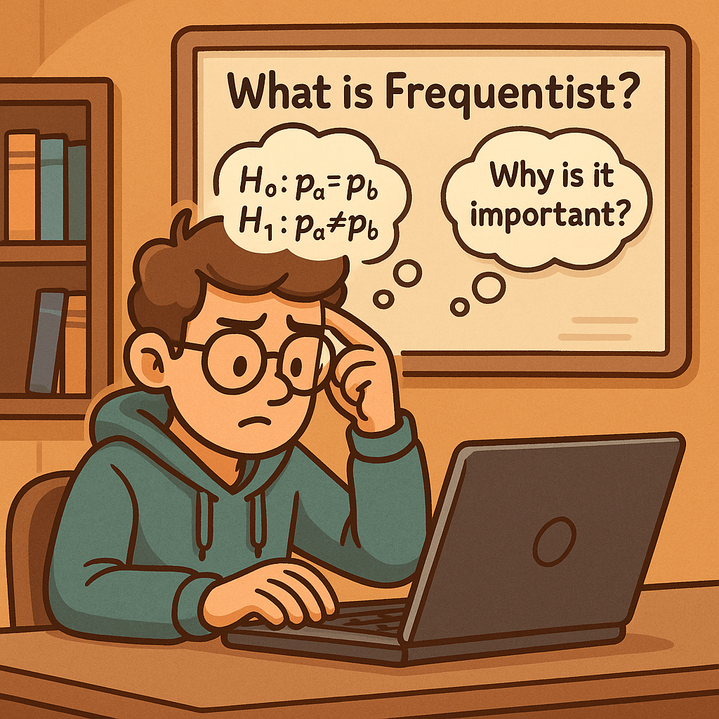
What is “Frequentist” in A/B Testing?

Frequentist inference interprets probability as the long-run frequency of events. In the context of A/B tests, it asks: If I repeatedly ran this experiment under the null hypothesis, how often would I observe a result at least this extreme just by chance?
Key objects in the frequentist toolkit are null/alternative hypotheses, test statistics, p-values, confidence intervals, Type I/II errors, and power.

Core Concepts (Fast Definitions)

• Null hypothesis (H₀): No difference between variants (e.g., p_A=p_B​).
• Alternative hypothesis (H₁): There is a difference (two-sided) or a specified direction (one-sided).
• Test statistic: A standardized measure (e.g., a z-score) used to compare observed effects to what chance would produce.
• p-value: Probability, assuming H₀ is true, of observing data at least as extreme as what you saw.
• Significance level (α): Threshold for rejecting H₀ (often 0.05).
• Confidence interval (CI): A range of plausible values for the effect size that would capture the true effect in X% of repeated samples.
• Power (1−β): Probability your test detects a true effect of a specified size (i.e., avoids a Type II error).

How Frequentist A/B Testing Works (Step-by-Step)

1) Define the effect and hypotheses

For a proportion metric like conversion rate (CR):

• p_A​ = baseline CR (variant A/control)
• p_B​ = treatment CR (variant B/experiment)

Null hypothesis:

$H{0}_{}:pA=pB$

Two-sided alternative:

$H{1}_{}:pA\ne pB$

2) Choose α, power, and (optionally) the Minimum Detectable Effect (MDE)

• Common choices: α = 0.05, power = 0.8 or 0.9.
• MDE is the smallest lift you care to detect (planning parameter for sample size).

3) Collect data according to a pre-registered plan

Let n_A,n_B​ be samples; x_A,x_B​ conversions; p_A=x_A/n_A, p_B=x_B/n_B.

4) Compute the test statistic (two-proportion z-test)

Pooled proportion under H₀:

$p=\frac{xA+xB}{nA+nB}$

Standard error (SE) under H₀:

$\mathrm{SE}=\sqrt{p(1-p)\times (\frac{1}{n}+\frac{1}{n})}$

z-statistic:

$z=\frac{(pB-pA)}{\mathrm{SE}}$

5) Convert z to a p-value

For a two-sided test:

$\text{p−value}=2\times (1-\Phi (\mid z\mid \left)\right)$

where Φ is the standard normal CDF.

6) Decision rule

• If p-value ≤ α ⇒ Reject H₀ (evidence of a difference).
• If p-value > α ⇒ Fail to reject H₀ (data are consistent with no detectable difference).

7) Report the effect size with a confidence interval

Approximate 95% CI for the difference (p_B−p_A):

$(pB-pA)\pm 1.96\times \sqrt{\frac{p}{}nA+\frac{p}{}nB}$

Tip: Also report relative lift (p_B/p_A−1) and absolute difference (p_B−p_A).

A Concrete Example (Conversions)

Suppose:

• n_A=10,000,  x_A=900⇒p_A=0.09
• n_B=10,000,  x_B=960⇒p_B=0.096

Compute pooled p​, SE, z, p-value, CI using the formulas above. If the two-sided p-value ≤ 0.05 and the CI excludes 0, you can conclude a statistically significant lift of ~0.6 percentage points (≈6.7% relative).

Why Frequentist Testing Is Important

1. Clear, widely-understood decisions
   Frequentist tests provide a familiar yes/no decision rule (reject/fail to reject H₀) that is easy to operationalize in product pipelines.
2. Error control at scale
   By fixing α, you control the long-run rate of false positives (Type I errors), crucial when many teams run many tests.

$\text{TypeIerrorrate}=\alpha$

3. Confidence intervals communicate uncertainty
   CIs provide a range of plausible effects, helping stakeholders gauge practical significance (not just p-values).
4. Power planning avoids underpowered tests
   You can plan sample sizes to hit desired power for your MDE, reducing wasted time and inconclusive results.

Approximate two-sample proportion power-based sample size per variant:

$n\approx \frac{(z\text{1−α/2}\times \sqrt{2p(1-p)}+z\text{power}\times \sqrt{p(1-p)+\mathrm{(p+\Delta )}(1-p-\Delta )})}{{\Delta }^2}$

where p is baseline CR and Δ is your MDE in absolute terms.

Practical Guidance & Best Practices

• Pre-register your hypothesis, metrics, α, stopping rule, and analysis plan.
• Avoid peeking (optional stopping inflates false positives). If you need flexibility, use group-sequential or alpha-spending methods.
• Adjust for multiple comparisons when testing many variants/metrics (e.g., Bonferroni, Holm, or control FDR).
• Check metric distributional assumptions. For very small counts, prefer exact or mid-p tests; for large samples, z-tests are fine.
• Report both statistical and practical significance. A tiny but “significant” lift may not be worth the engineering cost.
• Monitor variance early. High variance metrics (e.g., revenue/user) may require non-parametric tests or transformations.

Frequentist vs. Bayesian

• Frequentist p-values tell you how unusual your data are if H₀ were true.
• Bayesian methods provide a posterior distribution for the effect (e.g., probability the lift > 0).
  Both are valid; frequentist tests remain popular for their simplicity, well-established error control, and broad tooling support.

Common Pitfalls & How to Avoid Them

• Misinterpreting p-values: A p-value is not the probability H₀ is true.
• Multiple peeks without correction: Inflates Type I errors—use planned looks or sequential methods.
• Underpowered tests: Leads to inconclusive results—plan with MDE and power.
• Metric shift & novelty effects: Run long enough to capture stabilized user behavior.
• Winner’s curse: Significant early winners may regress—replicate or run holdout validation.

Reporting Template

• Hypothesis: H₀:p_A=p_B, H₁​: two-sided
• Design: α=0.05, power=0.8, MDE=…
• Data: n_A,x_A,p_A; n_B,x_B,p_B
• Analysis: two-proportion z-test (pooled), 95% CI
• Result: p-value = …, z = …, 95% CI = […, …], effect = absolute … / relative …
• Decision: reject/fail to reject H₀
• Notes: peeking policy, multiple-test adjustments, assumptions check

Final Takeaway

Frequentist A/B testing gives you a disciplined framework to decide whether a product change truly moves your metric or if the observed lift could be random noise. With clear error control, simple decision rules, and mature tooling, it remains a workhorse for experimentation at scale.