Search

Software Engineer's Notes

Month

October 2025

What Is CAPTCHA? Understanding the Gatekeeper of the Web

What Is CAPTCHA? Understanding the Gatekeeper of the Web

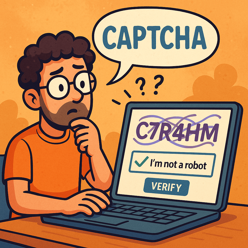
CAPTCHA — an acronym for Completely Automated Public Turing test to tell Computers and Humans Apart — is one of the most widely used security mechanisms on the internet. It acts as a digital gatekeeper, ensuring that users interacting with a website are real humans and not automated bots. From login forms to comment sections and online registrations, CAPTCHA helps maintain the integrity of digital interactions.

The History of CAPTCHA

The concept of CAPTCHA was first introduced in the early 2000s by a team of researchers at Carnegie Mellon University, including Luis von Ahn, Manuel Blum, Nicholas Hopper, and John Langford.

Their goal was to create a test that computers couldn’t solve easily but humans could — a reverse Turing test. The original CAPTCHAs involved distorted text images that required human interpretation.

Over time, as optical character recognition (OCR) technology improved, CAPTCHAs had to evolve to stay effective. This led to the creation of new types, including:

  • Image-based CAPTCHAs: Users select images matching a prompt (e.g., “Select all images with traffic lights”).
  • Audio CAPTCHAs: Useful for visually impaired users, playing distorted audio that needs transcription.
  • reCAPTCHA (2007): Acquired by Google in 2009, this variant helped digitize books and later evolved into reCAPTCHA v2 (“I’m not a robot” checkbox) and v3, which uses risk analysis based on user behavior.

Today, CAPTCHAs have become an essential part of web security and user verification worldwide.

How Does CAPTCHA Work?

At its core, CAPTCHA works by presenting a task that is easy for humans but difficult for bots. The system leverages differences in human cognitive perception versus machine algorithms.

The Basic Flow:

  1. Challenge Generation:
    The server generates a random challenge (e.g., distorted text, pattern, image selection).
  2. User Interaction:
    The user attempts to solve it (e.g., typing the shown text, identifying images).
  3. Verification:
    The response is validated against the correct answer stored on the server or verified using a third-party CAPTCHA API.
  4. Access Granted/Denied:
    If correct, the user continues the process; otherwise, the system requests another attempt.

Modern CAPTCHAs like reCAPTCHA v3 use behavioral analysis — tracking user movements, mouse patterns, and browsing behavior — to determine whether the entity is human without explicit interaction.

Why Do We Need CAPTCHA?

CAPTCHAs serve as a first line of defense against malicious automation and spam. Common scenarios include:

  • Preventing spam comments on blogs or forums.
  • Protecting registration and login forms from brute-force attacks.
  • Securing online polls and surveys from manipulation.
  • Protecting e-commerce checkouts from fraudulent bots.
  • Ensuring fair access to services like ticket booking or limited-edition product launches.

Without CAPTCHA, automated scripts could easily overload or exploit web systems, leading to security breaches, data misuse, and infrastructure abuse.

Challenges and Limitations of CAPTCHA

While effective, CAPTCHAs also introduce several challenges:

  • Accessibility Issues:
    Visually impaired users or users with cognitive disabilities may struggle with complex CAPTCHAs.
  • User Frustration:
    Repeated or hard-to-read CAPTCHAs can hurt user experience and increase bounce rates.
  • AI Improvements:
    Modern AI models, especially those using machine vision, can now solve traditional CAPTCHAs with >95% accuracy, forcing constant innovation.
  • Privacy Concerns:
    Some versions (like reCAPTCHA) rely on user behavior tracking, raising privacy debates.

Developers must balance security, accessibility, and usability when implementing CAPTCHA systems.

Real-World Examples

Here are some examples of CAPTCHA usage in real applications:

  • Google reCAPTCHA – Used across millions of websites to protect forms and authentication flows.
  • Cloudflare Turnstile – A privacy-focused alternative that verifies users without tracking.
  • hCaptcha – Offers website owners a reward model while verifying human interactions.
  • Ticketmaster – Uses CAPTCHA during high-demand sales to prevent bots from hoarding tickets.
  • Facebook and Twitter – Employ CAPTCHAs to block spam accounts and fake registrations.

Integrating CAPTCHA into Modern Software Development

Integrating CAPTCHA into your development workflow can be straightforward, especially with third-party APIs and libraries.

Step-by-Step Integration Example (Google reCAPTCHA v2):

  1. Register your site at Google reCAPTCHA Admin Console.
  2. Get the site key and secret key.
  3. Add the CAPTCHA widget in your frontend form:
<pre class="wp-block-syntaxhighlighter-code"><form action="verify.php" method="post">
  <div class="g-recaptcha" data-sitekey="YOUR_SITE_KEY"></div>
  <input type="submit" value="Submit">
</form>
<a href="https://www.google.com/recaptcha/api.js">https://www.google.com/recaptcha/api.js</a>
</pre>
  1. Verify the response in your backend (e.g., PHP, Python, Java):
import requests

response = requests.post(
    "https://www.google.com/recaptcha/api/siteverify",
    data={"secret": "YOUR_SECRET_KEY", "response": user_response}
)
result = response.json()
if result["success"]:
    print("Human verified!")
else:
    print("Bot detected!")

  1. Handle verification results appropriately in your application logic.

Integration Tips:

  • Combine CAPTCHA with rate limiting and IP reputation analysis for stronger security.
  • For accessibility, always provide audio or alternate options.
  • Use asynchronous validation to improve UX.
  • Avoid placing CAPTCHA on every form unnecessarily — use it strategically.

Conclusion

CAPTCHA remains a cornerstone of online security — balancing usability and protection. As automation and AI evolve, so must CAPTCHA systems. The shift from simple text challenges to behavior-based and privacy-preserving verification illustrates this evolution.

For developers, integrating CAPTCHA thoughtfully into the software development process can significantly reduce automated abuse while maintaining a smooth user experience.

MemorySanitizer (MSan): A Practical Guide for Finding Uninitialized Memory Reads

What is MemorySanitizer ?

What is MemorySanitizer?

MemorySanitizer (MSan) is a runtime instrumentation tool that flags reads of uninitialized memory in C/C++ (and languages that compile down to native code via Clang/LLVM). Unlike AddressSanitizer (ASan), which focuses on heap/stack/global buffer overflows and use-after-free, MSan’s sole mission is to detect when your program uses a value that was never initialized (e.g., a stack variable you forgot to set, padding bytes in a struct, or memory returned by malloc that you used before writing to it).

Common bug patterns MSan catches:

  • Reading a stack variable before assignment.
  • Using struct/class fields that are conditionally initialized.
  • Consuming library outputs that contain undefined bytes.
  • Leaking uninitialized padding across ABI boundaries.
  • Copying uninitialized memory and later branching on it.

How does MemorySanitizer work?

At a high level:

  1. Compiler instrumentation
    When you compile with -fsanitize=memory, Clang inserts checks and metadata propagation into your binary. Every program byte that could hold a runtime value gets an associated “shadow” state describing whether that value is initialized (defined) or not (poisoned).
  2. Shadow memory & poisoning
    • Shadow memory is a parallel memory space that tracks definedness of each byte in your program’s memory.
    • When you allocate memory (stack/heap), MSan poisons it (marks as uninitialized).
    • When you assign to memory, MSan unpoisons the relevant bytes.
    • When you read memory, MSan checks the shadow. If any bit is poisoned, it reports an uninitialized read.
  3. Taint/propagation
    Uninitialized data is treated like a taint: if you compute z = x + y and either x or y is poisoned, then z becomes poisoned. If poisoned data controls a branch or system call parameter, MSan reports it.
  4. Intercepted library calls
    Many libc/libc++ functions are intercepted so MSan can maintain correct shadow semantics—for example, telling MSan that memset to a constant unpoisons bytes, or that read() fills a buffer with defined data (or not, depending on return value). Using un-instrumented libraries breaks these guarantees (see “Issues & Pitfalls”).
  5. Origin tracking (optional but recommended)
    With -fsanitize-memory-track-origins=2, MSan stores an origin stack trace for poisoned values. When a bug triggers, you’ll see both:
    • Where the uninitialized read happens, and
    • Where the data first became poisoned (e.g., the stack frame where a variable was allocated but never initialized).
      This dramatically reduces time-to-fix.

Key Components (in detail)

  1. Compiler flags
    • Core: -fsanitize=memory
    • Origins: -fsanitize-memory-track-origins=2 (levels: 0/1/2; higher = richer origin info, more overhead)
    • Typical extras: -fno-omit-frame-pointer -g -O1 (or your preferred -O level; keep debuginfo for good stacks)
  2. Runtime library & interceptors
    MSan ships a runtime that:
    • Manages shadow/origin memory.
    • Intercepts popular libc/libc++ functions, syscalls, threading primitives, etc., to keep shadow state accurate.
  3. Shadow & Origin Memory
    • Shadow: tracks definedness per byte.
    • Origin: associates poisoned bytes with a traceable “birthplace” (function/file/line), invaluable for root cause.
  4. Reports & Stack Traces
    When MSan detects an uninitialized read, it prints:
    • The site of the read (file:line stack).
    • The origin (if enabled).
    • Register/memory dump highlighting poisoned bytes.
  5. Suppressions & Options
    • You can use suppressions for known noisy functions or third-party libs you cannot rebuild.
    • Runtime tuning via env vars (e.g., MSAN_OPTIONS) to adjust reporting, intercept behaviors, etc.

Issues, Limitations, and Gotchas

  • You must rebuild (almost) everything with MSan.
    If any library is not compiled with -fsanitize=memory (and proper flags), its interactions may produce false positives or miss bugs. This is the #1 hurdle.
    • In practice, you rebuild your app, its internal libraries, and as many third-party libs as feasible.
    • For system libs where rebuild is impractical, rely on interceptors and suppressions, but expect gaps.
  • Platform support is narrower than ASan.
    MSan primarily targets Linux and specific architectures. It’s less ubiquitous than ASan or UBSan. (Check your Clang/LLVM version’s docs for exact support.)
  • Runtime overhead.
    Expect ~2–3× CPU overhead and increased memory consumption, more with origin tracking. MSan is intended for CI/test builds—not production.
  • Focus scope: uninitialized reads only.
    MSan won’t detect buffer overflows, UAF, data races, UB patterns, etc. Combine with ASan/TSan/UBSan in separate jobs.
  • Struct padding & ABI wrinkles.
    Padding bytes frequently remain uninitialized and can “escape” via I/O, hashing, or serialization. MSan will flag these—sometimes noisy, but often uncovering real defects (e.g., nondeterministic hashes).

How and When Should We Use MSan?

Use MSan when:

  • You have flaky tests or heisenbugs suggestive of uninitialized data.
  • You want strong guarantees that values used in logic/branches/syscalls were actually initialized.
  • You’re developing security-sensitive or determinism-critical code (crypto, serialization, compilers, DB engines).
  • You’re modernizing a legacy codebase known to rely on “it happens to work”.

Workflow advice:

  • Run MSan in dedicated CI jobs on debug or rel-with-debinfo builds.
  • Combine with high-coverage tests, fuzzers, and scenario suites.
  • Keep origin tracking enabled in at least one job.
  • Incrementally port third-party deps or apply suppressions as you go.

FAQ

Q: Can I run MSan in production?
A: Not recommended. The overhead is significant and the goal is pre-production bug finding.

Q: What if I can’t rebuild a system library?
A: Try a source build, fall back to MSan interceptors and suppressions, or write wrappers that fully initialize buffers before/after calls.

Q: How does MSan compare to Valgrind/Memcheck?
A: MSan is compiler-based and much faster, but requires recompilation. Memcheck is binary-level (no recompile) but slower; using both in different pipelines is often valuable.

Conclusion

MemorySanitizer is laser-focused on a class of bugs that can be subtle, security-relevant, and notoriously hard to reproduce. With a dedicated CI job, origin tracking, and disciplined rebuilds of dependencies, MSan will pay for itself quickly—turning “it sometimes fails” into a concrete stack trace and a one-line fix.

Sample Ratio Mismatch (SRM) in A/B Testing

What is Sample Ratio Mismatch?

What is Sample Ratio Mismatch?

Sample Ratio Mismatch (SRM) is when the observed allocation of users to variants differs significantly from the planned allocation.
Example: You configured a 50/50 split, but after 10,000 users you see 5,300 in A and 4,700 in B. That’s likely SRM.

SRM means the randomization or eligibility pipeline is biased (or data capture is broken), so any effect estimates (lift, p-values, etc.) can’t be trusted.

How SRM Works (Conceptually)

When you specify a target split like 50/50 or 33/33/34, each incoming unit (user, device, session, etc.) should be randomly bucketed so that the expected distribution matches your target in expectation.

Formally, for a test with k variants and total N assigned units, the expected count for variant i is:

E_i = p_i N

where

p_i is the target proportion for variant 𝑖 i and N

is the total sample size.

If the observed counts,

O_i

, differ from the expected more than chance alone would allow, you have an SRM.

How to Identify SRM (Step-by-Step)

1) Use a Chi-Square Goodness-of-Fit Test (recommended)

For k variants, compute:

χ2 = ( (O_iE_i)2 E_i )

with degrees of freedom df=k−1. Compute the p-value from the chi-square distribution. If the p-value is very small (common thresholds: 10−3 to 10−6), you’ve likely got an SRM.

Example (two-arm 50/50):
N=10,000,  OA=5,300,  OB=4,700,  EA=EB=5,000

χ2 = (5300-5000)^2 5000 + (4700-5000)^2 5000 =36

With df=1, p≈1.97×10⁻⁹. This triggers SRM.

2) Visual/Operational Checks

  • Live split dashboard: Show observed vs. expected % by variant.
  • Stratified checks: Repeat the chi-square by country, device, browser, app version, traffic source, time-of-day to find where the skew originates.
  • Time series: Plot cumulative allocation over time—SRM that “drifts” may indicate a rollout, caching, or traffic-mix issue.

3) Early-Warning Rule of Thumb

If your observed proportion deviates from the target by more than a few standard errors early in the test, investigate. For two arms with target p=0.5, the sampling variance under perfect randomization is:

σp = p(1p) N

Large persistent deviations → likely SRM.

Common Causes of SRM

  1. Eligibility asymmetry: Filters (geo, device, login state, new vs. returning) applied after assignment or applied differently per variant.
  2. Randomization at the wrong unit: Assigning by session but analyzing by user (or vice versa); cross-device users collide.
  3. Inconsistent hashing/salts: Different hash salt/seed per service or per page; some code paths skip/override the assignment.
  4. Sticky sessions / caching / CDNs: Edge caching or load balancer stickiness pinning certain users to one variant.
  5. Traffic shaping / rollouts: Feature flags, canary releases, or time-based rollouts inadvertently biasing traffic into one arm.
  6. Bot or test traffic: Non-human or QA traffic not evenly distributed (or filtered in one arm only).
  7. Telemetry loss / logging gaps: Events dropped more in one arm (ad-blockers, blocked endpoints, CORS, mobile SDK bugs).
  8. User-ID vs. device-ID mismatch: Some users bucketed by cookie, others by account ID; cookie churn changes ratios.
  9. Late triggers: Assignment happens at “conversion event” time in one arm but at page load in another.
  10. Geo or platform routing differences: App vs. web, iOS vs. Android, or specific regions routed to different infrastructure.

How to Prevent SRM (Design & Implementation)

  • Choose the right unit of randomization (usually user). Keep it consistent from assignment through analysis.
  • Server-side assignment with deterministic hashing on a stable ID (e.g., user_id). Example mapping:
b= { A if (H(user\_id||salt)modM)<pM B otherwise }

where H is a stable hash, M a large modulus (e.g., 106), and p the target proportion for A.

  • Single source of truth for assignment (SDKs/services call the same bucketing service).
  • Pre-exposure assignment: Decide the variant before any UI/network differences occur.
  • Symmetric eligibility: Apply identical inclusion/exclusion filters before assignment.
  • Consistent rollout & flags: If you use gradual rollouts, do it outside the experiment or symmetrically across arms.
  • Bot/QA filtering: Detect and exclude bots and internal IPs equally for all arms.
  • Observability: Log (unit_id, assigned_arm, timestamp, eligibility_flags, platform, geo) to a central stream. Monitor split, by segment, in real time.
  • Fail-fast alerts: Trigger alerts when SRM p-value falls below a strict threshold (e.g., p<10−4).

How to Fix SRM (Triage & Remediation)

  1. Pause the experiment immediately. Do not interpret effect estimates from an SRM-affected test.
  2. Localize the bias. Recompute chi-square by segment (geo, device, source). The segment with the strongest SRM often points to the root cause.
  3. Audit the assignment path.
    • Verify the unit ID is consistent (user_id vs. cookie).
    • Check hash function + salt are identical everywhere.
    • Ensure assignment occurs pre-render and isn’t skipped due to timeouts.
  4. Check eligibility filters. Confirm identical filters are applied before assignment and in both arms.
  5. Review infra & delivery. Look for sticky sessions, CDN cache keys, or feature flag rollouts that differ by arm.
  6. Inspect telemetry. Compare event loss rates by arm/platform. Fix SDK/network issues (e.g., batch size, retry logic, CORS).
  7. Sanitize traffic. Exclude bots/internal traffic uniformly; re-run SRM checks.
  8. Rerun a smoke test. After fixes, run a small, short dry-run experiment to confirm the split is healthy (no SRM) before relaunching the real test.

Analyst’s Toolkit (Ready-to-Use)

  • SRM Chi-Square (two-arm 50/50):
χ2 = (O_AN/2)2 N/2 + (O_BN/2)2 N/2
  • General kkk-arm expected counts:
E_i=p_iN
  • Standard error for a two-arm proportion (target ppp):
σp= p(1p) N

Practical Checklist

  • Confirm unit of randomization and use stable IDs.
  • Perform server-side deterministic hashing with shared salt.
  • Apply eligibility before assignment, symmetrically.
  • Exclude bots/QA consistently.
  • Instrument SRM alerts (e.g., chi-square p<10−4).
  • Segment SRM monitoring by platform/geo/source/time.
  • Pause & investigate immediately if SRM triggers.

Summary

SRM isn’t a minor annoyance—it’s a stop sign. It tells you that the randomization or measurement is broken, which can fabricate uplifts or hide regressions. Detect it early with a chi-square test, design your experiments to prevent it (stable IDs, deterministic hashing, symmetric eligibility), and never ship decisions from an SRM-affected test.

Unit of Randomization in A/B Testing: A Practical Guide

What is unit of randomization?

What is a “Unit of Randomization”?

The unit of randomization is the entity you randomly assign to variants (A or B). It’s the “thing” that receives the treatment: a user, a session, a device, a household, a store, a geographic region, etc.

Choosing this unit determines:

  • Who gets which experience
  • How independence assumptions hold (or break)
  • How you compute statistics and sample size
  • How actionable and unbiased your results are

How It Works (at a high level)

  1. Define exposure: decide what entity must see a consistent experience (e.g., “Logged-in user must always see the same variant across visits.”).
  2. Create an ID: select an identifier for that unit (e.g., user_id, device_id, household_id, store_id).
  3. Hash & assign: use a stable hashing function to map each ID into variant A or B with desired split (e.g., 50/50).
  4. Persist: ensure the unit sticks to its assigned variant on every exposure (stable bucketing).
  5. Analyze accordingly: aggregate metrics at or above the unit level; use the right variance model (especially for clusters).

Common Units of Randomization (with pros/cons and when to use)

1) User-Level (Account ID or Login ID)

  • What it is: Each unique user/account is assigned to a variant.
  • Use when: Logged-in products; experiences should persist across devices and sessions.
  • Pros: Clean independence between users; avoids cross-device contamination for logged-in flows.
  • Cons: Requires reliable, unique IDs; guest traffic may be excluded or need fallback logic.

2) Device-Level (Device ID / Mobile Advertiser ID)

  • What it is: Each physical device is assigned.
  • Use when: Native apps; no login, but device ID is stable.
  • Pros: Better than cookies for persistence; good for app experiments.
  • Cons: Same human on multiple devices may see different variants; may bias human-level metrics.

3) Cookie-Level (Browser Cookie)

  • What it is: Each browser cookie gets a variant.
  • Use when: Anonymous web traffic without login.
  • Pros: Simple to implement.
  • Cons: Cookies expire/clear; users have multiple browsers/devices → contamination and assignment churn.

4) Session-Level

  • What it is: Each session is randomized; the same user may see different variants across sessions.
  • Use when: You intentionally want short-lived treatment (e.g., page layout in a one-off landing funnel).
  • Pros: Fast ramp, lots of independent observations.
  • Cons: Violates persistence; learning/carryover effects make interpretation tricky for longer journeys.

5) Pageview/Request-Level

  • What it is: Every pageview or API request is randomized.
  • Use when: Low-stakes UI tweaks with negligible carryover; ads/creative rotation tests.
  • Pros: Maximum volume quickly.
  • Cons: Massive contamination; not suitable when the experience should be consistent within a visit.

6) Household-Level

  • What it is: All members/devices of a household share the same assignment (derived from address or shared account).
  • Use when: TV/streaming, grocery delivery, multi-user homes.
  • Pros: Limits within-home interference; aligns with purchase behavior.
  • Cons: Hard to define reliably; potential privacy constraints.

7) Network/Team/Organization-Level

  • What it is: Randomize at a group/organization level (e.g., company admin sets a feature; all employees see it).
  • Use when: B2B products; settings that affect the whole group.
  • Pros: Avoids spillovers inside an org.
  • Cons: Fewer units → lower statistical power; requires cluster-aware analysis.

8) Geographic/Store/Region-Level (Cluster Randomization)

  • What it is: Entire locations are assigned (cities, stores, countries, data centers).
  • Use when: Pricing, inventory, logistics, or features tied to physical/geo constraints.
  • Pros: Realistic operational measurement, cleaner separation across regions.
  • Cons: Correlated outcomes within a cluster; requires cluster-robust analysis and typically larger sample sizes.

Why the Unit of Randomization Matters

1) Validity (Independence & Interference)

Statistical tests assume independent observations. If people in the control are affected by those in treatment (interference), estimates are biased. Picking a unit that contains spillovers (e.g., randomize at org or store level) preserves validity.

2) Power & Sample Size (Design Effect)

Clustered units (households, stores, orgs) share similarities—captured by intra-class correlation (ICC), often denoted ρ\rhoρ. This inflates variance via the design effect:

DE = 1 + ( m 1 ) ρ

Where m is the average cluster size. Your effective sample size becomes:

neff = n DE

Larger clusters or higher ρ → bigger DE → less power for the same raw n.

3) Consistency of Experience

Units like user-level + stable bucketing ensure a user’s experience doesn’t flip between variants, avoiding dilution and confusion.

4) Interpretability & Actionability

If you sell at the store level, store-level randomization makes metrics easier to translate into operational decisions. If you optimize user engagement, user-level makes more sense.

How to Choose the Right Unit (Decision Checklist)

  • Where do spillovers happen?
    Pick the smallest unit that contains meaningful interference (user ↔ household ↔ org ↔ region).
  • What is the primary decision maker?
    If rollouts happen per account/org/region, align the unit with that boundary.
  • Can you persist assignment?
    Use stable identifiers and hashing (e.g., SHA-256 on user_id + experiment_name) to keep assignments sticky.
  • How will you analyze it?
    • User/cookie/device: standard two-sample tests aggregated per unit.
    • Cluster (org/store/geo): use cluster-robust standard errors or mixed-effects models; adjust for design effect in planning.
  • Is the ID reliable & unique?
    Prefer user_id over cookie when possible. If only cookies exist, add fallbacks and measure churn.

Practical Implementation Tips

  • Stable Bucketing: Hash the chosen unit ID to a uniform number in [0,1); map ranges to variants (e.g., <0.5 → A, ≥0.5 → B). Store assignment server-side for reliability.
  • Cross-Device Consistency: If the same human might use multiple devices, prefer user-level (requires login) or implement a linking strategy (e.g., email capture) before randomization.
  • Exposure Control: Ensure treatment is only applied after assignment; log exposures to avoid partial-treatment bias.
  • Metric Aggregation: Aggregate outcomes per randomized unit first (e.g., user-level conversion), then compare arms. Avoid pageview-level analysis when randomizing at user level.
  • Bot & Duplicate Filtering: Scrub bots and detect duplicate IDs (e.g., shared cookies) to reduce contamination.
  • Pre-Experiment Checks: Verify balance on key covariates (traffic source, device, geography) across variants for the chosen unit.

Examples

  • Pricing test in retail chain → randomize at store level; compute sales per store; analyze with cluster-robust errors; account for region seasonality.
  • New signup flow on a web app → randomize at user level (or cookie if anonymous); ensure users see the same variant across sessions.
  • Homepage hero image rotation for paid ads landing page → potentially session or pageview level; keep awareness of contamination if users return.

Common Pitfalls (and how to avoid them)

  • Using too granular a unit (pageview) for features with memory/carryover → inconsistent experiences and biased results.
    Fix: move to session or user level.
  • Ignoring clustering when randomizing stores/teams → inflated false positives.
    Fix: use cluster-aware analysis and plan for design effect.
  • Cookie churn breaks persistence → variant switching mid-experiment.
    Fix: server-side assignment with long-lived identifiers; encourage login.
  • Interference across units (social/network effects) → contamination.
    Fix: enlarge the unit (household/org/region) or use geo-experiments with guard zones.

Frequentist Inference in A/B Testing: A Practical Guide

What is Frequentist ?

What is “Frequentist” in A/B Testing?

Frequentist inference interprets probability as the long-run frequency of events. In the context of A/B tests, it asks: If I repeatedly ran this experiment under the null hypothesis, how often would I observe a result at least this extreme just by chance?
Key objects in the frequentist toolkit are null/alternative hypotheses, test statistics, p-values, confidence intervals, Type I/II errors, and power.

Core Concepts (Fast Definitions)

  • Null hypothesis (H₀): No difference between variants (e.g., pA=pB​).
  • Alternative hypothesis (H₁): There is a difference (two-sided) or a specified direction (one-sided).
  • Test statistic: A standardized measure (e.g., a z-score) used to compare observed effects to what chance would produce.
  • p-value: Probability, assuming H₀ is true, of observing data at least as extreme as what you saw.
  • Significance level (α): Threshold for rejecting H₀ (often 0.05).
  • Confidence interval (CI): A range of plausible values for the effect size that would capture the true effect in X% of repeated samples.
  • Power (1−β): Probability your test detects a true effect of a specified size (i.e., avoids a Type II error).

How Frequentist A/B Testing Works (Step-by-Step)

1) Define the effect and hypotheses

For a proportion metric like conversion rate (CR):

  • pA​ = baseline CR (variant A/control)
  • pB​ = treatment CR (variant B/experiment)

Null hypothesis:

H0:pA=pB

Two-sided alternative:

H1:pApB

2) Choose α, power, and (optionally) the Minimum Detectable Effect (MDE)

  • Common choices: α = 0.05, power = 0.8 or 0.9.
  • MDE is the smallest lift you care to detect (planning parameter for sample size).

3) Collect data according to a pre-registered plan

Let nA,nB​ be samples; xA,xB​ conversions; pA=xA/nA, pB=xB/nB.

4) Compute the test statistic (two-proportion z-test)

Pooled proportion under H₀:

p=xA+xBnA+nB

Standard error (SE) under H₀:

SE=p(1p)×(1nA+1nB)

z-statistic:

z=(pBpA)SE

5) Convert z to a p-value

For a two-sided test:

p−value=2×(1Φ(z))

where Φ is the standard normal CDF.

6) Decision rule

  • If p-value ≤ α ⇒ Reject H₀ (evidence of a difference).
  • If p-value > α ⇒ Fail to reject H₀ (data are consistent with no detectable difference).

7) Report the effect size with a confidence interval

Approximate 95% CI for the difference (pB−pA):

(pBpA)±1.96×pA(1pA)nA+pB(1pB)nB

Tip: Also report relative lift (pB/pA−1) and absolute difference (pB−pA).

A Concrete Example (Conversions)

Suppose:

  • nA=10,000,  xA=900⇒pA=0.09
  • nB=10,000,  xB=960⇒pB=0.096

Compute pooled p​, SE, z, p-value, CI using the formulas above. If the two-sided p-value ≤ 0.05 and the CI excludes 0, you can conclude a statistically significant lift of ~0.6 percentage points (≈6.7% relative).

Why Frequentist Testing Is Important

  1. Clear, widely-understood decisions
    Frequentist tests provide a familiar yes/no decision rule (reject/fail to reject H₀) that is easy to operationalize in product pipelines.
  2. Error control at scale
    By fixing α, you control the long-run rate of false positives (Type I errors), crucial when many teams run many tests.
TypeIerrorrate=α
  1. Confidence intervals communicate uncertainty
    CIs provide a range of plausible effects, helping stakeholders gauge practical significance (not just p-values).
  2. Power planning avoids underpowered tests
    You can plan sample sizes to hit desired power for your MDE, reducing wasted time and inconclusive results.

Approximate two-sample proportion power-based sample size per variant:

n(z1−α/2×2p(1p)+z power×p(1p)+(p+Δ)(1pΔ))Δ2

where p is baseline CR and Δ is your MDE in absolute terms.

Practical Guidance & Best Practices

  • Pre-register your hypothesis, metrics, α, stopping rule, and analysis plan.
  • Avoid peeking (optional stopping inflates false positives). If you need flexibility, use group-sequential or alpha-spending methods.
  • Adjust for multiple comparisons when testing many variants/metrics (e.g., Bonferroni, Holm, or control FDR).
  • Check metric distributional assumptions. For very small counts, prefer exact or mid-p tests; for large samples, z-tests are fine.
  • Report both statistical and practical significance. A tiny but “significant” lift may not be worth the engineering cost.
  • Monitor variance early. High variance metrics (e.g., revenue/user) may require non-parametric tests or transformations.

Frequentist vs. Bayesian

  • Frequentist p-values tell you how unusual your data are if H₀ were true.
  • Bayesian methods provide a posterior distribution for the effect (e.g., probability the lift > 0).
    Both are valid; frequentist tests remain popular for their simplicity, well-established error control, and broad tooling support.

Common Pitfalls & How to Avoid Them

  • Misinterpreting p-values: A p-value is not the probability H₀ is true.
  • Multiple peeks without correction: Inflates Type I errors—use planned looks or sequential methods.
  • Underpowered tests: Leads to inconclusive results—plan with MDE and power.
  • Metric shift & novelty effects: Run long enough to capture stabilized user behavior.
  • Winner’s curse: Significant early winners may regress—replicate or run holdout validation.

Reporting Template

  • Hypothesis: H0:pA=pB, H1​: two-sided
  • Design: α=0.05, power=0.8, MDE=…
  • Data: nA,xA,pA; nB,xB,pB
  • Analysis: two-proportion z-test (pooled), 95% CI
  • Result: p-value = …, z = …, 95% CI = […, …], effect = absolute … / relative …
  • Decision: reject/fail to reject H₀
  • Notes: peeking policy, multiple-test adjustments, assumptions check

Final Takeaway

Frequentist A/B testing gives you a disciplined framework to decide whether a product change truly moves your metric or if the observed lift could be random noise. With clear error control, simple decision rules, and mature tooling, it remains a workhorse for experimentation at scale.

Stable Bucketing in A/B Testing

What is Stable Bucketing?

What Is Stable Bucketing?

Stable bucketing is a repeatable, deterministic way to assign units (users, sessions, accounts, devices, etc.) to experiment variants so that the same unit always lands in the same bucket whenever the assignment is recomputed. It’s typically implemented with a hash function over a unit identifier and an experiment “seed” (or namespace), then mapped to a bucket index.

Key idea: assignment never changes for a given (unit_id, experiment_seed) unless you deliberately change the seed or unit of bucketing. This consistency is crucial for clean experiment analysis and operational simplicity.

Why We Need It (At a Glance)

  • Consistency: Users don’t flip between A and B when they return later.
  • Reproducibility: You can recompute assignments offline for debugging and analysis.
  • Scalability: Works statelessly across services and languages.
  • Safety: Lets you ramp traffic up or down without re-randomizing previously assigned users.
  • Analytics integrity: Reduces bias and cross-contamination when users see multiple experiments.

How Stable Bucketing Works (Step-by-Step)

1) Choose Your Unit of Bucketing

Pick the identity that best matches the causal surface of your treatment:

  • User ID (most common): stable across sessions/devices (if you have login).
  • Device ID: when login is rare; beware of cross-device spillover.
  • Session ID / Request ID: only for per-request or per-session treatments.

Rule of thumb: bucket at the level where the treatment is applied and outcomes are measured.

2) Build a Deterministic Hash

Compute a hash over a canonical string like:

canonical_key = experiment_namespace + ":" + unit_id
hash = H(canonical_key)  // e.g., 64-bit MurmurHash3, xxHash, SipHash

Desiderata: fast, language-portable implementations, low bias, and uniform output over a large integer space (e.g., 2^64).

3) Normalize to [0, 1)

Convert the integer hash to a unit interval. With a 64-bit unsigned hash h∈{0,…,264−1}:

u = h / 2^64   // floating-point in [0,1)

4) Map to Buckets

If you have K total buckets (e.g., 1000) and want to allocate N of them to the experiment (others remain “control” or “not in experiment”), you can map:

bucket = u × K

Then assign variant ranges. For a 50/50 split with two variants A and B over the same experiment allocation, for example:

  • A gets buckets [0,K/2−1]
  • B gets buckets [K/2,K−1]

You can also reserve a global “control” by giving it a fixed bucket range that is outside any experiment’s allocation.

5) Control Allocation (Traffic Percentage)

If the intended inclusion probability is p (e.g., 10%), assign the first p⋅K buckets to the experiment:

N = p × K

Include a unit if bucket < N. Split inside N across variants according to desired proportions.

Minimal Pseudocode (Language-Agnostic)

function assign_variant(unit_id, namespace, variants):
    // variants = [{name: "A", weight: 0.5}, {name: "B", weight: 0.5}]
    key = namespace + ":" + canonicalize(unit_id)
    h = Hash64(key)                       // e.g., MurmurHash3 64-bit
    u = h / 2^64                          // float in [0,1)
    // cumulative weights to pick variant
    cum = 0.0
    for v in variants:
        cum += v.weight
        if u < cum:
            return v.name
    return variants[-1].name              // fallback for rounding

Deterministic: same (unit_id, namespace) → same u → same variant every time.

Statistical Properties (Why It Works)

Assuming the hash behaves like a uniform random function over [0,1), the inclusion indicator li​ for each unit i with target probability p is:

(A) = E[n_A] = pn Var[n_A] = np(1p)

With stable bucketing, units included at ramp-up remain included as you increase p (monotone ramps), which avoids re-randomization noise.

Benefits & Why It’s Important (In Detail)

1) User Experience Consistency

  • A returning user continues to see the same treatment, preventing confusion and contamination.
  • Supports long-running or incremental rollouts (10% → 25% → 50% → 100%) without users flipping between variants.

2) Clean Causal Inference

  • Avoids cross-over effects that can bias estimates when users switch variants mid-experiment.
  • Ensures SUTVA-like stability at the chosen unit (no unit’s potential outcomes change due to assignment instability).

3) Operational Simplicity & Scale

  • Stateless assignment (derive on the fly from (unit_id, namespace)).
  • Works across microservices and languages as long as the hash function and namespace are shared.

4) Reproducibility & Debugging

  • Offline recomputation lets you verify assignments, investigate suspected sample ratio mismatches (SRM), and audit exposure logs.

5) Safe Traffic Management

  • Ramps: increasing p simply widens the bucket interval—no reshuffling of already exposed users.
  • Kill-switches: setting p=0 instantly halts new exposures while keeping analysis intact.

6) Multi-Experiment Harmony

  • Use namespaces or layered bucketing to keep unrelated experiments independent while permitting intended interactions when needed.

Practical Design Choices & Pitfalls

Hash Function

  • Prefer fast, well-tested non-cryptographic hashes (MurmurHash3, xxHash).
  • If adversarial manipulation is a risk (e.g., public IDs), consider SipHash or SHA-based hashing.

Namespace (Seed) Discipline

  • The experiment_namespace must be unique per experiment/phase. Changing it intentionally re-randomizes.
  • For follow-up experiments requiring independence, use a new namespace. For continued exposure, reuse the old one.

Bucket Count & Mapping

  • Use a large K (e.g., 10,000) to get fine-grained control over traffic percentages and reduce allocation rounding issues.

Unit of Bucketing Mismatch

  • If treatment acts at the user level but you bucket by device, a single user on two devices can see different variants (spillover). Align unit with treatment.

Identity Resolution

  • Cross-device/user-merges can change effective unit IDs. Decide whether to lock assignment post-merge or recompute at login—document the policy and its analytical implications.

SRM Monitoring

  • Even with stable bucketing, instrumentation bugs, filters, and eligibility rules can create SRM. Continuously monitor observed splits versus expected ppp.

Privacy & Compliance

  • Hash only pseudonymous identifiers and avoid embedding raw PII in logs. Salt/namespace prevents reuse of the same hash across experiments.

Example: Two-Variant 50/50 with 20% Traffic

Setup

  • K=10,000 buckets
  • Experiment gets p=0.2 ⇒ N=2,000 buckets
  • Within experiment, A and B each get 50% of the N buckets (1,000 each)

Mapping

  • Include user if 0 ≤ bucket < 2000
  • If included:
    • A: 0 ≤ bucket < 1000
    • B: 1000 ≤ bucket < 2000
  • Else: not in experiment (falls through to global control)

Ramp from 20% → 40%

  • Extend inclusion to 0 ≤ bucket < 4000
  • Previously included users stay included; new users are added without reshuffling earlier assignments.

Math Summary (Allocation & Variant Pick)

Inclusion Decision

include = [ u×K < N ]

Variant Selection by Cumulative Weights

Let variants have weights w1,…wm​ with ∑wj=1 . Pick the smallest j such that:

u < k=1 wk

Implementation Tips (Prod-Ready)

  • Canonicalization: Lowercase IDs, trim whitespace, and normalize encodings before hashing.
  • Language parity tests: Create cross-language golden tests (input → expected bucket) for your SDKs.
  • Versioning: Version your bucketing algorithm; log algo_version, namespace, and unit_id_type.
  • Exposure logs: Record (unit_id, namespace, variant, timestamp) for auditability.
  • Dry-run: Add an endpoint or feature flag to validate expected split on synthetic data before rollout.

Takeaways

Stable bucketing is the backbone of reliable A/B testing infrastructure. By hashing a stable unit ID within a disciplined namespace, you get deterministic, scalable, and analyzable assignments. This prevents cross-over effects, simplifies rollouts, and preserves statistical validity—exactly what you need for trustworthy product decisions.

Minimum Detectable Effect (MDE) in A/B Testing

What is minimum detectable effect?

In the world of A/B testing, precision and statistical rigor are essential to ensure that our experiments deliver meaningful and actionable results. One of the most critical parameters in designing an effective experiment is the Minimum Detectable Effect (MDE). Understanding what MDE is, how it works, and why it matters can make the difference between a successful data-driven decision and a misleading one.

What is Minimum Detectable Effect?

The Minimum Detectable Effect (MDE) represents the smallest difference between a control group and a variant that an experiment can reliably detect as statistically significant.

In simpler terms, it’s the smallest change in your key metric (such as conversion rate, click-through rate, or average order value) that your test can identify with confidence — given your chosen sample size, significance level, and statistical power.

If the real effect is smaller than the MDE, the test is unlikely to detect it, even if it truly exists.

How Does It Work?

To understand how MDE works, let’s start by looking at the components that influence it. MDE is mathematically connected to sample size, statistical power, significance level (α), and data variability (σ).

The basic idea is this:

A smaller MDE means you can detect tiny differences between variants, but it requires a larger sample size. Conversely, a larger MDE means you can detect only big differences, but you’ll need fewer samples.

Formally, the relationship can be expressed as follows:

MDE = z(1α/2) + z(power) n × σ

Where:

  • MDE = Minimum Detectable Effect
  • z(1−α/2) = critical z-score for the chosen confidence level
  • z(power) = z-score corresponding to desired statistical power
  • σ = standard deviation (data variability)
  • n = sample size per group

Main Components of MDE

Let’s break down the main components that influence MDE:

1. Significance Level (α)

The significance level represents the probability of rejecting the null hypothesis when it is actually true (a Type I error).
A common value is α = 0.05, which corresponds to a 95% confidence level.
Lowering α (for more stringent tests) increases the z-score, making the MDE larger unless you also increase your sample size.

2. Statistical Power (1−β)

Power is the probability of correctly rejecting the null hypothesis when there truly is an effect (avoiding a Type II error).
Commonly, power is set to 0.8 (80%) or 0.9 (90%).
Higher power makes your test more sensitive — but also demands more participants for the same MDE.

3. Variability (σ)

The standard deviation (σ) of your data reflects how much individual observations vary from the mean.
High variability makes it harder to detect differences, thus increasing the required MDE or the sample size.

For example, conversion rates with wide daily fluctuations will require a larger sample to confidently detect a small change.

4. Sample Size (n)

The sample size per group is one of the most controllable factors in experiment design.
Larger samples provide more statistical precision and allow for smaller detectable effects (lower MDE).
However, larger samples also mean longer test durations and higher operational costs.

Example Calculation

Let’s assume we are running an A/B test on a website with the following parameters:

  • Baseline conversion rate = 5%
  • Desired power = 80%
  • Significance level (α) = 0.05
  • Standard deviation (σ) = 0.02
  • Sample size (per group) = 10,000

Plugging these values into the MDE equation:

MDE = 1.96+0.84 10000 × 0.02 MDE = 2.8 100 × 0.02 = 0.00056 = 0.056%

This means our test can detect at least a 0.056% improvement in conversion rate with the given parameters.

Why is MDE Important?

MDE is fundamental to experimental design because it connects business expectations with statistical feasibility.

  • It ensures your experiment is neither underpowered nor wasteful.
  • It helps you balance test sensitivity and resource allocation.
  • It prevents false assumptions about the test’s ability to detect meaningful effects.
  • It informs stakeholders about what level of improvement is measurable and realistic.

In practice, if your expected effect size is smaller than the calculated MDE, you may need to increase your sample size or extend the test duration to achieve reliable results.

Integrating MDE into Your A/B Testing Process

When planning A/B tests, always define the MDE upfront — alongside your confidence level, power, and test duration.
Most modern experimentation platforms allow you to input these parameters and will automatically calculate the required sample size.

A good practice is to:

  1. Estimate your baseline metric and expected improvement.
  2. Compute the MDE using the formulas above.
  3. Adjust your test duration or audience accordingly.
  4. Validate assumptions post-test to ensure the MDE was realistic.

Conclusion

The Minimum Detectable Effect (MDE) is the cornerstone of statistically sound A/B testing.
By understanding and applying MDE correctly, you can design experiments that are both efficient and credible — ensuring that the insights you draw truly reflect meaningful improvements in your product or business.

A/B Testing: A Practical Guide for Software Teams

What is A/B Testing?

What Is A/B Testing?

A/B testing (a.k.a. split testing or controlled online experiments) is a method of comparing two or more variants of a product change—such as copy, layout, flow, pricing, or algorithm—by randomly assigning users to variants and measuring which one performs better against a predefined metric (e.g., conversion, retention, time-to-task).

At its heart: random assignment + consistent tracking + statistical inference.

A Brief History (Why A/B Testing Took Over)

  • Early 1900s — Controlled experiments: Agricultural and medical fields formalized randomized trials and statistical inference.
  • Mid-20th century — Statistical tooling: Hypothesis testing, p-values, confidence intervals, power analysis, and experimental design matured in academia and industry R&D.
  • 1990s–2000s — The web goes measurable: Log files, cookies, and analytics made user behavior observable at scale.
  • 2000s–2010s — Experimentation platforms: Companies productized experimentation (feature flags, automated randomization, online metrics pipelines).
  • Today — “Experimentation culture”: Product, growth, design, and engineering teams treat experiments as routine, from copy tweaks to search/recommendation algorithms.

Core Components & Features

1) Hypothesis & Success Metrics

  • Hypothesis: A clear, falsifiable statement (e.g., “Showing social proof will increase sign-ups by 5%”).
  • Primary metric: One north-star KPI (e.g., conversion rate, revenue/user, task completion).
  • Guardrail metrics: Health checks to prevent harm (e.g., latency, churn, error rates).

2) Randomization & Assignment

  • Unit of randomization: User, session, account, device, or geo—pick the unit that minimizes interference.
  • Stable bucketing: Deterministic hashing (e.g., userID → bucket) ensures users stay in the same variant.
  • Traffic allocation: 50/50 is common; you can ramp gradually (1% → 5% → 20% → 50% → 100%).

3) Instrumentation & Data Quality

  • Event tracking: Consistent event names, schemas, and timestamps.
  • Exposure logging: Record which variant each user saw.
  • Sample Ratio Mismatch (SRM) checks: Detect broken randomization or filtering errors.

4) Statistical Engine

  • Frequentist or Bayesian: Both are valid; choose one approach and document your decision rules.
  • Power & duration: Estimate sample size before launch to avoid underpowered tests.
  • Multiple testing controls: Correct when running many metrics or variants.

5) Feature Flagging & Rollouts

  • Kill switch: Instantly turn off a harmful variant.
  • Targeting: Scope by country, device, cohort, or feature entitlement.
  • Gradual rollouts: Reduce risk and observe leading indicators.

How A/B Testing Works (Step-by-Step)

  1. Frame the problem
    • Define the user problem and the behavioral outcome you want to change.
    • Write a precise hypothesis and pick one primary metric (and guardrails).
  2. Design the experiment
    • Choose the unit of randomization and traffic split.
    • Compute minimum detectable effect (MDE) and sample size/power.
    • Decide the test window (consider seasonality, weekends vs weekdays).
  3. Prepare instrumentation
    • Add/verify events and parameters.
    • Add exposure logging (user → variant).
    • Set up dashboards for primary and guardrail metrics.
  4. Implement variants
    • A (control): Current experience.
    • B (treatment): Single, intentionally scoped change. Avoid bundling many changes.
  5. Ramp safely
    • Start with a small percentage to validate no obvious regressions (guardrails: latency, errors, crash rate).
    • Increase to planned split once stable.
  6. Run until stopping criteria
    • Precommit rules: fixed sample size or statistical thresholds (e.g., 95% confidence / high posterior).
    • Don’t peek and stop early unless you’ve planned sequential monitoring.
  7. Analyze & interpret
    • Check SRM, data freshness, assignment integrity.
    • Evaluate effect size, uncertainty (CIs or posteriors), and guardrails.
    • Consider heterogeneity (e.g., new vs returning users), but beware p-hacking.
  8. Decide & roll out
    • Ship B if it improves the primary metric without harming guardrails.
    • Rollback or iterate if neutral/negative or inconclusive.
    • Document learnings and add to a searchable “experiment logbook.”

Benefits

  • Customer-centric outcomes: Real user behavior, not opinions.
  • Reduced risk: Gradual exposure with kill switches prevents widespread harm.
  • Compounding learning: Your experiment log becomes a strategic asset.
  • Cross-functional alignment: Designers, PMs, and engineers align around clear metrics.
  • Efficient investment: Double down on changes that actually move the needle.

Challenges & Pitfalls (and How to Avoid Them)

  • Underpowered tests: Too little traffic or too short duration → inconclusive results.
    • Fix: Do power analysis; increase traffic or MDE; run longer.
  • Sample Ratio Mismatch (SRM): Unequal assignment when you expected 50/50.
    • Fix: Automate SRM checks; verify hashing, filters, bot traffic, and eligibility gating.
  • Peeking & p-hacking: Repeated looks inflate false positives.
    • Fix: Predefine stopping rules; use sequential methods if you must monitor continuously.
  • Metric mis-specification: Optimizing vanity metrics can hurt long-term value.
    • Fix: Choose metrics tied to business value; set guardrails.
  • Interference & contamination: Users see both variants (multi-device) or influence each other (network effects).
    • Fix: Pick the right unit; consider cluster-randomized tests.
  • Seasonality & novelty effects: Short-term lifts can fade.
    • Fix: Run long enough; validate with holdouts/longitudinal analysis.
  • Multiple comparisons: Many metrics/variants inflate Type I error.
    • Fix: Pre-register metrics; correct (e.g., Holm-Bonferroni) or use hierarchical/Bayesian models.

When Should You Use A/B Testing?

Use it when:

  • You can randomize exposure and measure outcomes reliably.
  • The expected effect is detectable with your traffic and time constraints.
  • The change is reversible and safe to ramp behind a flag.
  • You need causal evidence (vs. observational analytics).

Avoid or rethink when:

  • The feature is safety-critical or legally constrained (no risky variants).
  • Traffic is too low for a meaningful test—consider switchback tests, quasi-experiments, or qualitative research.
  • The change is broad and coupled (e.g., entire redesign) — consider staged launches plus targeted experiments inside the redesign.

Integrating A/B Testing Into Your Software Development Process

1) Add Experimentation to Your SDLC

  • Backlog (Idea → Hypothesis):
    • Each experiment ticket includes hypothesis, primary metric, MDE, power estimate, and rollout plan.
  • Design & Tech Spec:
    • Define variants, event schema, exposure logging, and guardrails.
    • Document assignment unit and eligibility filters.
  • Implementation:
    • Wrap changes in feature flags with a kill switch.
    • Add analytics events; verify in dev/staging with synthetic users.
  • Code Review:
    • Check flag usage, deterministic bucketing, and event coverage.
    • Ensure no variant leaks (CSS/JS not loaded across variants unintentionally).
  • Release & Ramp:
    • Start at 1–5% to validate stability; then ramp to target split.
    • Monitor guardrails in real time; alert on SRM or error spikes.
  • Analysis & Decision:
    • Use precommitted rules; share dashboards; write a brief “experiment memo.”
    • Update your Experiment Logbook (title, hypothesis, dates, cohorts, results, learnings, links to PRs/dashboards).
  • Operationalize Learnings:
    • Roll proven improvements to 100%.
    • Create Design & Content Playbooks from repeatable wins (e.g., messaging patterns that consistently outperform).

2) Minimal Tech Stack (Tool-Agnostic)

  • Feature flags & targeting: Server-side or client-side SDK with deterministic hashing.
  • Assignment & exposure service: Central place to decide variant and log the exposure event.
  • Analytics pipeline: Event ingestion → cleaning → sessionization/cohorting → metrics store.
  • Experiment service: Defines experiments, splits traffic, enforces eligibility, and exposes results.
  • Dashboards & alerting: Real-time guardrails + end-of-test summaries.
  • Data quality jobs: Automated SRM checks, missing event detection, and schema validation.

3) Governance & Culture

  • Pre-registration: Write hypotheses and metrics before launch.
  • Ethics & privacy: Respect consent, data minimization, and regional regulations.
  • Education: Train PM/Design/Eng on power, peeking, SRM, and metric selection.
  • Review board (optional): Larger orgs can use a small reviewer group to sanity-check experimental design.

Practical Examples

  • Signup flow: Test shorter forms vs. progressive disclosure; primary metric: completed signups; guardrails: support tickets, refund rate.
  • Onboarding: Compare tutorial variants; metric: 7-day activation (first “aha” event).
  • Pricing & packaging: Test plan names or anchor prices in a sandboxed flow; guardrails: churn, support contacts, NPS.
  • Search/ranking: Algorithmic tweaks; use interleaving or bucket testing with holdout cohorts; guardrails: latency, relevance complaints.

FAQ

Q: Frequentist or Bayesian?
A: Either works if you predefine decision rules and educate stakeholders. Bayesian posteriors are intuitive; frequentist tests are widely standard.

Q: How long should I run a test?
A: Until you reach the planned sample size or stopping boundary, covering at least one full user-behavior cycle (e.g., weekend + weekday).

Q: What if my traffic is low?
A: Increase MDE, test higher-impact changes, aggregate across geos, or use sequential tests. Complement with qualitative research.

Quick Checklist

  • Hypothesis, primary metric, guardrails, MDE, power
  • Unit of randomization and eligibility
  • Feature flag + kill switch
  • Exposure logging and event schema
  • SRM monitoring and guardrail alerts
  • Precommitted stopping rules
  • Analysis report + decision + logbook entry

End-to-End Testing in Software Development

What is End to End testing?

In today’s fast-paced software world, ensuring your application works seamlessly from start to finish is critical. That’s where End-to-End (E2E) testing comes into play. It validates the entire flow of an application — from the user interface down to the database and back — making sure every component interacts correctly and the overall system meets user expectations.

What is End-to-End Testing?

End-to-End testing is a type of software testing that evaluates an application’s workflow from start to finish, simulating real-world user scenarios. The goal is to verify that the entire system — including external dependencies like databases, APIs, and third-party services — functions correctly together.

Instead of testing a single module or service in isolation, E2E testing ensures that the complete system behaves as expected when all integrated parts are combined.

For example, in an e-commerce system:

  • A user logs in,
  • Searches for a product,
  • Adds it to the cart,
  • Checks out using a payment gateway,
  • And receives a confirmation email.

E2E testing verifies that this entire sequence works flawlessly.

How Does End-to-End Testing Work?

End-to-End testing typically follows these steps:

  1. Identify User Scenarios
    Define the critical user journeys — the sequences of actions users perform in real life.
  2. Set Up the Test Environment
    Prepare a controlled environment that includes all necessary systems, APIs, and databases.
  3. Define Input Data and Expected Results
    Determine what inputs will be used and what the expected output or behavior should be.
  4. Execute the Test
    Simulate the actual user actions step by step using automated or manual scripts.
  5. Validate Outcomes
    Compare the actual behavior against expected results to confirm whether the test passes or fails.
  6. Report and Fix Issues
    Log any discrepancies and collaborate with the development team to address defects.

Main Components of End-to-End Testing

Let’s break down the key components that make up an effective E2E testing process:

1. Test Scenarios

These represent real-world user workflows. Each scenario tests a complete path through the system, ensuring functional correctness across modules.

2. Test Data

Reliable, representative test data is crucial. It mimics real user inputs and system states to produce accurate testing results.

3. Test Environment

A controlled setup that replicates the production environment — including databases, APIs, servers, and third-party systems — to validate integration behavior.

4. Automation Framework

Automation tools such as Cypress, Selenium, Playwright, or TestCafe are often used to run tests efficiently and repeatedly.

5. Assertions and Validation

Assertions verify that the actual output matches the expected result. These validations ensure each step in the workflow behaves correctly.

6. Reporting and Monitoring

After execution, results are compiled into reports for developers and QA engineers to analyze, helping identify defects quickly.

Benefits of End-to-End Testing

1. Ensures System Reliability

By testing complete workflows, E2E tests ensure that the entire application — not just individual components — works as intended.

2. Detects Integration Issues Early

Since E2E testing validates interactions between modules, it can catch integration bugs that unit or component tests might miss.

3. Improves User Experience

It simulates how real users interact with the system, guaranteeing that the most common paths are always functional.

4. Increases Confidence Before Release

With E2E testing, teams gain confidence that new code changes won’t break existing workflows.

5. Reduces Production Failures

Because it validates real-life scenarios, E2E testing minimizes the risk of major failures after deployment.

Challenges of End-to-End Testing

While E2E testing offers significant value, it also comes with some challenges:

  1. High Maintenance Cost
    Automated E2E tests can become fragile as UI or workflows change frequently.
  2. Slow Execution Time
    Full workflow tests take longer to run than unit or integration tests.
  3. Complex Setup
    Simulating a full production environment — with multiple services, APIs, and databases — can be complex and resource-intensive.
  4. Flaky Tests
    Tests may fail intermittently due to timing issues, network delays, or dependency unavailability.
  5. Difficult Debugging
    When something fails, tracing the root cause can be challenging since multiple systems are involved.

When and How to Use End-to-End Testing

E2E testing is best used when:

  • Critical user workflows need validation.
  • Cross-module integrations exist.
  • Major releases are scheduled.
  • You want confidence in production stability.

Typically, it’s conducted after unit and integration tests have passed.
In Agile or CI/CD environments, E2E tests are often automated and run before deployment to ensure regressions are caught early.

Integrating End-to-End Testing into Your Software Development Process

Here’s how you can effectively integrate E2E testing:

  1. Define Key User Journeys Early
    Collaborate with QA, developers, and business stakeholders to identify essential workflows.
  2. Automate with Modern Tools
    Use frameworks like Cypress, Selenium, or Playwright to automate repetitive E2E scenarios.
  3. Incorporate into CI/CD Pipeline
    Run E2E tests automatically as part of your build and deployment process.
  4. Use Staging Environments
    Always test in an environment that mirrors production as closely as possible.
  5. Monitor and Maintain Tests
    Regularly update test scripts as the UI, APIs, and workflows evolve.
  6. Combine with Other Testing Levels
    Balance E2E testing with unit, integration, and acceptance testing to maintain a healthy test pyramid.

Conclusion

End-to-End testing plays a vital role in ensuring the overall quality and reliability of modern software applications.
By validating real user workflows, it gives teams confidence that everything — from UI to backend — functions smoothly.

While it can be resource-heavy, integrating automated E2E testing within a CI/CD pipeline helps teams catch critical issues early and deliver stable, high-quality releases.

Blog at WordPress.com.

Up ↑