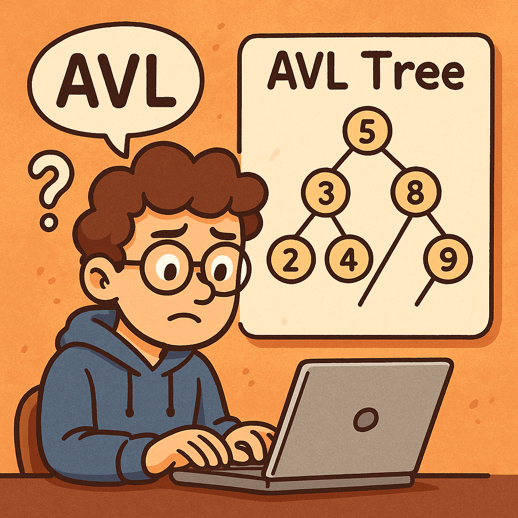
What is an AVL Tree?
An AVL tree (named after Adelson-Velsky and Landis) is a self-balancing Binary Search Tree (BST).
For every node, the balance factor (height of left subtree − height of right subtree) is constrained to −1, 0, or +1. When inserts or deletes break this rule, the tree rotates (LL, RR, LR, RL cases) to restore balance—keeping the height O(log n).
Key idea: By preventing the tree from becoming skewed, every search, insert, and delete stays fast and predictable.
When Do We Need It?
Use an AVL tree when you need ordered data with consistently fast lookups and you can afford a bit of extra work during updates:
- Read-heavy workloads where searches dominate (e.g., 90% reads / 10% writes)
- Realtime ranking/leaderboards where items must stay sorted
- In-memory indexes (e.g., IDs, timestamps) for low-latency search and range queries
- Autocomplete / prefix sets (when implemented over keys that must remain sorted)
Real-World Example
Imagine a price alert service maintaining thousands of stock tickers in memory, keyed by last-trade time.
- Every incoming request asks, “What changed most recently?” or “Find the first ticker after time T.”
- With an AVL tree, search and successor/predecessor queries remain O(log n) even during volatile trading, while rotations keep the structure balanced despite frequent inserts/deletes.
Main Operations and Complexity
Operations
- Search(k) – standard BST search
- Insert(k, v) – BST insert, then rebalance with rotations (LL, RR, LR, RL)
- Delete(k) – BST delete (may replace with predecessor/successor), then rebalance
- Find min/max, predecessor/successor, range queries
Time Complexity
- Search: O(log n)
- Insert: O(log n) (includes at most a couple of rotations)
- Delete: O(log n) (may trigger rotations)
- Min/Max, predecessor/successor: O(log n)
Space Complexity
- Space: O(n) for nodes
- Per-node overhead: O(1) (store height or balance factor)
Advantages
- Guaranteed O(log n) for lookup, insert, delete (tighter balance than many alternatives)
- Predictable latency under worst-case patterns (no pathologically skewed trees)
- Great for read-heavy or latency-sensitive workloads
Disadvantages
- More rotations/updates than looser trees (e.g., Red-Black) → slightly slower writes
- Implementation complexity (more cases to handle correctly)
- Cache locality worse than B-trees on disk; not ideal for large on-disk indexes
Quick Note on Rotations
- LL / RR: one single rotation fixes it
- LR / RL: a double rotation (child then parent) fixes it
Rotations are local (affect only a few nodes) and keep the BST order intact.
AVL vs. (Plain) Binary Tree — What’s the Difference?
Many say “binary tree” when they mean “binary search tree (BST).” A plain binary tree has no ordering or balancing guarantees.
An AVL is a BST + balance rule that keeps height logarithmic.
| Feature | Plain Binary Tree | Unbalanced BST | AVL (Self-Balancing BST) |
|---|---|---|---|
| Ordering of keys | Not required | In-order (left < node < right) | In-order (left < node < right) |
| Balancing rule | None | None | Height difference per node ∈ {−1,0,+1} |
| Worst-case height | O(n) | O(n) (e.g., sorted inserts) | O(log n) |
| Search | O(n) worst-case | O(n) worst-case | O(log n) |
| Insert/Delete | O(1)–O(n) | O(1)–O(n) | O(log n) (with rotations) |
| Update overhead | Minimal | Minimal | Moderate (rotations & height updates) |
| Best for | Simple trees/traversals | When input is random and small | Read-heavy, latency-sensitive, ordered data |
When to Prefer AVL Over Other Trees
- Choose AVL when you must keep lookups consistently fast and don’t mind extra work on writes.
- Choose Red-Black Tree when write throughput is a bit more important than the absolute tightness of balance.
- Choose B-tree/B+-tree for disk-backed or paged storage.
Minimal Insert (Pseudo-Java) for Intuition
class Node {
  int key, height;
  Node left, right;
}

int h(Node n){ return n==null?0:n.height; }
int bf(Node n){ return n==null?0:h(n.left)-h(n.right); }
void upd(Node n){ n.height = 1 + Math.max(h(n.left), h(n.right)); }

Node rotateRight(Node y){
  Node x = y.left, T2 = x.right;
  x.right = y; y.left = T2;
  upd(y); upd(x);
  return x;
}
Node rotateLeft(Node x){
  Node y = x.right, T2 = y.left;
  y.left = x; x.right = T2;
  upd(x); upd(y);
  return y;
}

Node insert(Node node, int key){
  if(node==null) return new Node(){ {this.key=key; this.height=1;} };
  if(key < node.key) node.left = insert(node.left, key);
  else if(key > node.key) node.right = insert(node.right, key);
  else return node; // no duplicates

  upd(node);
  int balance = bf(node);

  // LL
  if(balance > 1 && key < node.left.key) return rotateRight(node);
  // RR
  if(balance < -1 && key > node.right.key) return rotateLeft(node);
  // LR
  if(balance > 1 && key > node.left.key){ node.left = rotateLeft(node.left); return rotateRight(node); }
  // RL
  if(balance < -1 && key < node.right.key){ node.right = rotateRight(node.right); return rotateLeft(node); }

  return node;
}
Summary
- AVL = BST + strict balance → height O(log n)
- Predictable performance for search/insert/delete: O(log n)
- Best for read-heavy or latency-critical ordered data; costs a bit more on updates.
- Compared to a plain binary tree or unbalanced BST, AVL avoids worst-case slowdowns by design.
Recent Comments